Flow visualization

Compared to visualization of dynamical systems, much more work has been done in the field of flow visualization. Experimental and/or empirical techniques have already been used for quite a long time.

In recent time flow visualization increasingly is done one a computational basis. Fluid flows as well as gaseous flows are simulated in the research field of computational fluid dynamics (CFD). Often finite element methods are used to handle complex flow structures, for instance, local solvers of the Navier-Stokes equations, which work on various kinds of grids. Usually data sets are computed that provide a huge amount of sampled vector information spread over a two- or three-dimensional domain.

Without visualization it is usually impossible to reasonably investigate such data sets. At this point flow visualization comes into play. It already provides numerous techniques to view various properties of such huge data sets, e.g., turbulences, vortical structures, separation lines, etc.

  

Figure 2.3: Experimental flow visualization, two examples [67]:  (a) particles within the flow (image by Delft Hydraulics) and  (b) shadow graph technique (image by High-Speed Lab, Dept. of Aerospace Eng., Delft Univ. of Techn.).

Experimental and empirical approaches

For quite a long time, researchers who deal with flows are using experimental setups to get an impression of its properties and structures, to get ideas about improvements to their work, and/or to evaluate their models. Three basic types of experimental techniques can be distinguished [67]:

Adding foreign material -

Dye or magnesium powder is injected into liquid flow to visualize flow dynamics. See Fig. 2.3(a) for an example, where a model of a harbor was visualized using particles within the flow. In gaseous flows smoke or oil droplets are injected.

A problem with injecting material is that the injection process and the injected material may influence the flow. Using electrolytic techniques for generating hydrogen bubbles within the flow decreases these problems to a certain extent. Also photochemical methods are used, for instance, generating dye within the flow using a laser beam.

Applying tufts to the walls of a flow simulation, or coating certain border surfaces of interest with some viscous material like oil, visualizes flow behavior near objects within the flow, for example, flow close to aircraft wings in a wind tunnel.

Optical techniques -

less disturbence of the flow can be achieved using optical methods. Optical properties like light refraction change at places within the flow where there are big local differences in flow density. Working with a light beam, images are generated with shadows and caustics. See Fig. 2.3(b) for an example, where shadows in the image denote shock waves within the flow.

Another visual property which changes in regions of high density gradients, is the phase of light rays. Interferometry is an example of a technique which exploits such phase shifts.

Adding heat/energy -

heat can be applied to flows to artificially increase the density variation - optical techniques are then used for visualization. Shooting electrons into the flow volume is used to excite gas molecules. After being excited the molecules emit their extra energy as light particles, which visualizes flow patterns.

Although experimental methods have advantages - feedback is intuitive, no numerical errors, immediate response, etc. - there are some significant disadvantages: most severe is the fact, that experimental methods influence the flow itself. Next, experimental setups usually are time consuming and very expensive. Finally, there is just a limited set of flow properties that can be visualized using experimental techniques.

In addition to experimental methods, empirical techniques - flow patterns are drawn by hand after investigation - also have a long tradition. Leonardo da Vinci used hand drawings to communicate his research results on fluid flows. More recently, Abraham and Shaw came up with visualizing flow structures by using hand-drawn images [1].

For in-depth information about experimental flow visualization techniques, see Merzkirch [55], Yang [93], and van Dyke [85].

  

Figure 2.4: Three basic visualization techniques used for the Lotka-Volterra model:  (a) hedgehog plot,  (b) streamlets, and  (c) LIC.

Methods for two-dimensional flow fields

The less dimensions a dynamical system has, the easier visualization is. Techniques for the visualization of two-dimensional dynamical systems (or vector fields) already have quite a tradition in flow investigation. Hedgehog plots, also called arrow plots, usually show a large number of small arrows that indicate the flow direction at many (regularly spaced) points of the two-dimensional domain. Often arrows are normalized, so flow velocity is not encoded. This is, to prevent the display from overloading due to very long and overlapping arrows. See Fig. 2.4(a) for a hedgehog plot of the Lotka-Volterra model (see also Eq. 1.2).

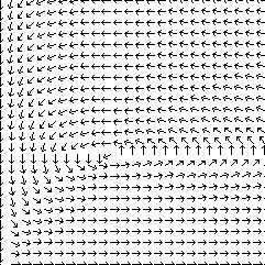
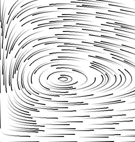
More elaborated are stream line graphs. The dynamical system or flow field is integrated numerically for some specific initial points. Depending on whether the flow is time-dependent or not, streak lines, path lines, or stream lines are generated [29]. Temporal correlation of virtual particles that are moved by the flow are intuitively depicted, such that an impression of the embedded dynamics can be gained quite intuitively. See Fig. 2.4(b) for a set of streamlets for the Lotka-Volterra model.

One problem with integral curves used in the visualization of continuous dynamical systems is the choice of the initial conditions. Evenly spaced seed points usually do not generate evenly spaced integral curves. Turk and Banks [84] and Jobard and Lefer [36,37] propose methods to cope with this problem and generate evenly spaced stream lines for two-dimensional flows.

Instead of placing many integral lines over the flow domain, texture-based methods, also provide very useful results. Spot noise by van Wijk [87,20] is generated by placing many small `spots', for example, elongated ellipses, on the flow domain and orienting them according to the local flow direction. Different intensities are chosen for the spots. Thereby a noise texture is generated which locally is correlated with flow direction. 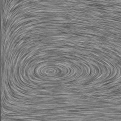Another texture-based technique, called line integral convolution (LIC) by Cabral and Leedom [14,23,24,78,79,90,89], generates similar results. A white noise texture is locally convoluted along flow trajectories. Again, a visual correlation along the flow is generated. Both techniques, spot noise and LIC, are capable of generating an overview of all the dynamics in a dynamical system. See Fig. 2.4(c) for a LIC image of the Lotka-Volterra system. Other techniques in this area are texture splats by Crawfis and Max [17], line bundles [16] and virtual ink droplets [48].

  

Figure 2.5: Two examples for rendering stream lines in 3D:  (a) illuminated stream lines by Zöckler et al. [94], and  (b) vector field rendering by Banks [8].

Direct visualization of 3D flows

In 3D the situation is more difficult than in 2D, since image synthesis involves a process of condensing visualization cues populating the three-dimensional domain. For example, arrow plots are usually not useful for three-dimensional flow, since depth perception of one-dimensional objects (the arrows) is poor compared to surface objects, and populating three-space with arrows easily produces overloaded images.

Representing stream lines as 1D curves, the use of stream lines or similar integral curves is difficult for the same reasons. Nevertheless, the intuitive understanding of this kind of direct representation of flow trajectories, i.e., of streamlets or stream lines, resulted in some interesting techniques, e.g., illuminated stream lines (cf. Fig. 2.5(a)) by Zöckler et al. [94] and vector field rendering (cf. Fig. 2.5(b)) by Banks [8].

  

Figure 2.6: Stream ribbons show the rotation around stream lines (image by Hans-Georg Pagendarm) [62].

Stream ribbons show, additional to flow paths, flow rotation around trajectories [29]. A stream line is integrated through the vector field. Additionally local surface elements are used to encode local flow rotation. Either a second trajectory is connected or differential analysis of the flow is used to compute the ribbon twist. Fig. 2.6 shows a visualization of oil flow patterns at the contact surface of the flow and stream ribbons within the flow used for vortex core visualization. In this image results of an experimental setup are overlaid with results from a CFD simulation of the same flow.

  

Figure 2.7: (a) Stream surface (image by the Data Visualization Group, NAS, NASA) [58].  (b) Flow volume (image by the Visualization group at LLNL) [18].

In addition to stream lines and stream ribbons, stream surfaces make up an important part of flow visualization in 3D. Instead of a point, one-dimensional sets of initial conditions are used in the vector field integration step. Hultquist described, how to compute stream surfaces for dynamics over a three-dimensional domain [33]. Problems with stream surfaces are, that extensive surface parts easily occlude other parts of the visualization, and missing information about flow direction and velocity within the stream surface. Chapter 4 describes stream arrows that might be used to decrease most of the problems apparent with stream surfaces. Fig. 2.7(a) shows an example of a stream surface.

Other integral objects than streamlets or stream lines are used for flow visualization also. Stream balls by Brill et al. [12] are based on the meta balls concept. A set of initial points (seed points) is used to define an iso-surface, i.e., the stream balls, using a potential field proportional to the distance from these seed points and some user-specified threshold value. Consequently the points are moved following the underlying vector field. Thereby new points are added to the initial set and a surface-like meta object is generated. In regions of local divergence the iso-surface separates into distinct sub-surfaces, whereas in regions of local convergence the iso-surfaces related to multiple points merge and built up a coherent meta object.

To investigate flow near boundary surfaces, virtual tufts are used. Short integral objects are computed with initial conditions next to boundary surfaces. Instead of stream surfaces, a particle system can be used for flow visualization [88]. Particles are modeled as small surface parts spread over the locus of a stream surface. Transparent areas in-between the particles reduce the problem of occlusion, while the particles still give a good impression of the stream surface. Particles are drawn as small ellipses. A normal vector assigned to each surface particle is used in shading calculations. Contrary to one- and two-dimensional visualization cues, flow volumes model the temporal evolution of an initial three-dimensional set [54]. This approach models the injection and propagation of smoke particles through the flow advection. Volume rendering is necessary to compute an image showing 3D flow visualized by the use of flow volumes. Local convergence or divergence is encoded by the density of the flow volume. Fig. 2.7(b) gives an example of a flow volume.

Visualizing local properties in 3D

Similar to dynamical systems flow data-sets also contain sub-sets of special interest. Vortex cores, for example, are very important structures in the simulation of flow around objects like airplanes, ships, turbines, etc [9,39]. In the case of dynamical systems separatrices are especially interesting. Because of their special importance these lower-dimensional structures often are investigated in more detail. Local properties that are derived from flow derivatives, i.e., the Jacobian matrices at states of interest, are also visualized.

  

Figure 2.8: Two examples for flow visualization by the use of stream tubes (images by Schröder et al. [75]).

One approach to the visualization of special trajectories together with their local properties are the stream polygon and stream tube techniques by Schröder et al. [75]. For a certain number of sample points along the stream line of interest, the Jacobian matrix is examined. A decomposition into a symmetric and an asymmetric part yields local rotational and shear information about the flow near the investigated trajectory. This information is mapped to the geometrical properties of polygons which are assumed to be normal to the flow direction. Size, shape, and rotation of the polygons illustrate local flow properties. By connecting the edges of adjacent stream polygons a stream tube is generated. In Fig. 2.8 two examples of stream tubes are shown.

  

Figure 2.9: (a) Local flow probe by de Leeuw and van Wijk [19].  (b) Icons for the visualization of local properties by Happe and Rumpf [74].

Even more `verbose' than stream polygon and stream tube, the local flow probe [19] by de Leeuw and van Wijk represents local flow properties also derived from the Jacobian matrix. Direction and orientation, velocity, acceleration, curvature, rotation, shear, and convergence/divergence of the flow near a special state of interest are mapped to distinct geometrical properties of a rather complex glyph. See Fig. 2.9(a) for a sample glyph generated with this technique. Placing several of these glyphs, for example, along an especially important trajectory, an intuitive visualization of local properties is provided.

Happe and Rumpf [74] extended the use of icons for representing local flow characteristics near critical points of the system. See Fig. 2.9(b) for a sample image generated using this technique. Post et al. also present advanced visualization techniques on the basis of icons [68].

  

Figure 2.10: Two examples of the visualization of vector field topology (images by Helman et al. [31]).

Visualizing the topology of vector fields

Helman and Hesselink [31] proposed to visualize the geometry of the topological structure of flow dynamics. Stream lines along the eigenvectors of critical points are used to show separatrices. Icons composed of line segments and small disks encode the Jacobian matrix near critical points. Globus et al. [27] came up with a tool to identify topological elements within data that is given at a discrete grid. Two sample images are shown in Fig. 2.10.

Overviews of work in this area are given by Levit in 1992 [43] and Asimov et al. in 1995 [7].

mailto:helwig@cg.tuwien.ac.at.