Rendering

Drawing 1D objects in 3D space poses several problems in the rendering stage. Shading, for example, improves the visual cues concerning the spatial arrangement of objects, but shading is usually defined on the basis of a surface (normal). In 3D lines and curves have an infinite number of normals at each of their points. Therefore typical shading models as Phong shading [64] can not be applied directly to 1D objects in 3D.

In 1989 Kajiya presented an ``ad hoc'' approach to deal with the problem of line shading in 3D which is based on an integration of all reflected intensities [38]. In 1996 Zöckler et al. described an efficient computation scheme for line shading in 3D which generates comparable results to the technique proposed by Kajiya [94]. A general framework for the task of shading k-manifolds in n-space was worked out by Banks in 1994 [8]. In addition to a consistent framework for shading with arbitrary co-dimensions Banks also dealt with the problem of excess brightness-compensation which becomes an important topic when manifolds with co-dimension higher than 1 are shaded.

Another problem associated with line shading in 3D is (self-)shadowing. Normally, when shading 2-manifolds in 3-space, we (implicitly) deal with this aspect by assuming all surface points in (self-)shadow, where the outward normal  n points away from the light vector  l, i.e.,  $\mathbf{n}\!\cdot\!\mathbf{l}<0$. Furthermore we consider shadow rays before we compute surface shading. Both aspects are difficult with line shading in 3D. One approach to deal with these aspects comes from volume rendering: lines populating certain regions of three-space can be considered as volume opacity of a certain density. This assumption yields an exponential brightness attenuation for light passing through such a region. A paper by Max in 1995 compiles a comprehensive list of diverse models dealing with this effect [53].

  

Figure 7.4: (a) A thread of streamlets visualizing the flow near a torus in 3D.  (b) Flow near a 3D focus visualized using two threads of streamlets.

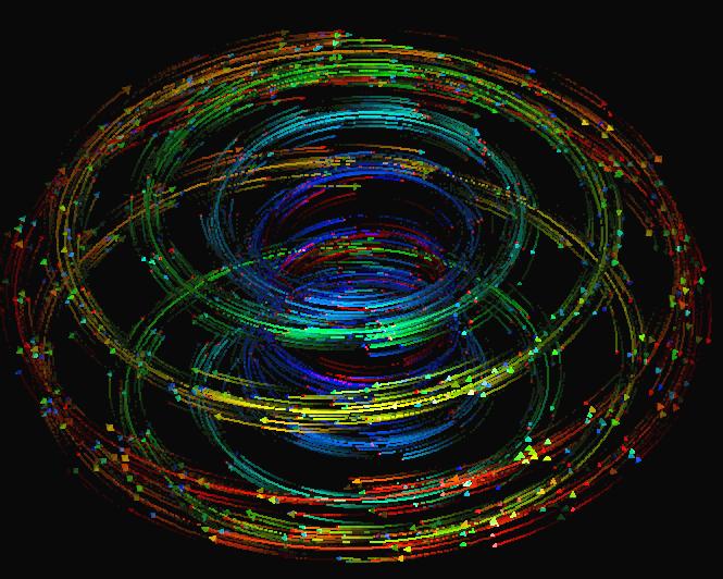
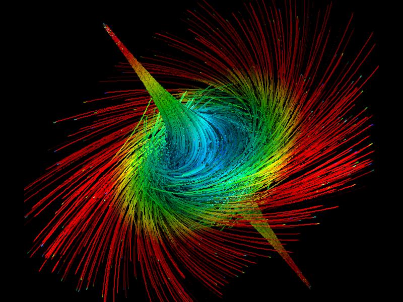
For the implementation of this technique the shading model by Zöckler was used for shading the streamlets. Additionally we used depth cueing as a rough approximation of shadowing to enhance the spatial perceptibility of the streamlets in three-space. See Fig. 7.4(a) for an example. The heads of the streamlets are represented by small arrow-heads to indicate the orientation of the flow. Color is used to encode the flow velocity (blue  $\leftrightarrow$ slow, red  $\leftrightarrow$ fast). Line shading and depth cueing has been applied as described above.

mailto:helwig@cg.tuwien.ac.at.