Results and Implementation

To test the technique we firstly applied it to a simple cases, i.e., the critical points of a linear dynamical system. Depending on the Jacobian matrix evaluated at this point, different results are obtained. Fig. 7.3(b) shows six threads of streamlets applied to the characteristic trajectories emanating from the critical point. In this case the eigenvalues of the Jacobian matrix at the critical point are 1, 10, and 100. The new visualization technique allows to easily depict the slow, medium, and fast directions of flow. Moreover, an impression is conveyed, how system states are repelled from the plane defined by the slow and medium direction (eigenvalues 1 and 10). Within that plane states are repelled from the slow direction which itself is therefore extremely instable in this setup. These flow characteristics typical for a dynamical system near a critical point cannot be communicated by either showing an abstraction only (Fig. 7.3(a)) or a complete set of stream lines.

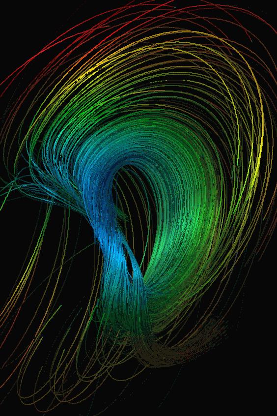
Fig. 7.4(b) is generated by using two threads of streamlets for the visualization of a 3D focus, of a linear dynamical system. The Jacobian matrix of this system exhibits one negative eigenvalue and two conjugated complex eigenvalues with positive real part. System states are attracted along an instable 1-manifold - a line in the case of a linear system - and repelled into a stable 2-manifold (plane) perpendicular to the instable set. Applying the threads to both instable trajectories the dynamics near this critical point are visualized. As in Fig. 7.4(a) color was used to encode flow velocity.

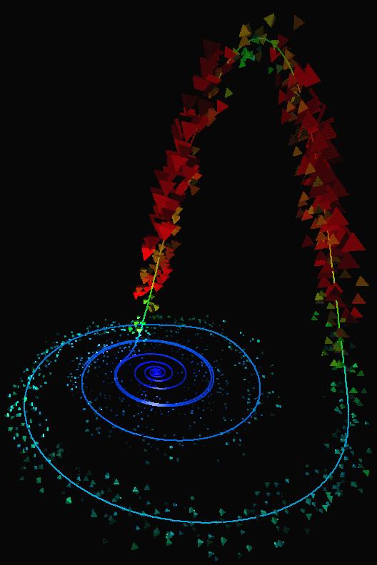
There is no restriction to apply the new technique to characteristic trajectories only. Fig. 7.5 shows two examples where different results where produced with this technique. The left image shows a thread of streamlets through the Roessler system. Instead of the streamlets themselves just arrow-heads at the end of each streamlets are displayed. Using size and color according to the velocity of the flow slow and fast areas within this system are visualized. The right image depicts the dynamics of a periodic flow near a twisted torus. Color coding indicates the velocity along the streamlets. In Fig. 7.5(a) and 7.5(b) no characteristic trajectories were used, the evolution of the streamlets is aligned with the base trajectory. Regions of local convergence/divergence are shown as areas with more/less streamlets.

  

Figure 7.5: (a) Visualizing the flow velocity near a stream line of the Roessler system.  (b) Visualizing the dynamics of a periodic dynamical system exhibiting a twisted torus.

The technique presented in this chapter was implemented within DynSys3D (see Chapter  8). The module generates one thread of streamlets for a specific dynamical system by using a specific numerical integrator. Parameters for the module are the starting location s of the base trajectory ( $\mathbf{s}\!=\!\mathcal{T}_\mathbf{s}(0)$) and its length (either temporal or spatial), the number of streamlets per cross-section ( $\mathit{no}$), the maximum distance of their seed-points (R) together with the fade-out parameter (q).

mailto:helwig@cg.tuwien.ac.at.