Figures - overview - Chapter 1


Figures - overview - Chapter 1 | |
| 1005-pite94-01-b.jpg, 1006-pite94-01-c.jpg |
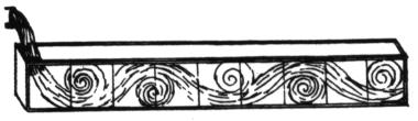
| Figure 1.1: Two examples of early flow visualization by Leonardo da Vinci (images out of ``Frontiers of Scientific Visualization'' by Pickover and Teksbury [65]). | |
| 1007-ppmodel1.gif, 1008-lvm-tailor.gif |
| Figure 1.2: (a) Cycles of evolution in 2D phase space, and (b) evolution of variable x over time t (both computed for a predator-prey model by Lotka/Volterra). | |
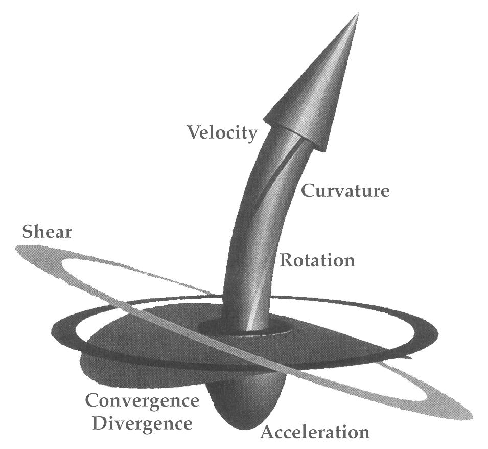
| 1009-class-b.gif |
| Figure 1.3: Different ways of viewing dynamical systems. | |
| 1010-class-vis.14.jpg, 1011-ds-vis.03.jpg |
| Figure 1.4: (a) Visualizing a 1D class of 1D dynamical systems - the parameter is varied along the horizontal axis. (b) Visualizing one specific 2D dynamical system. | |
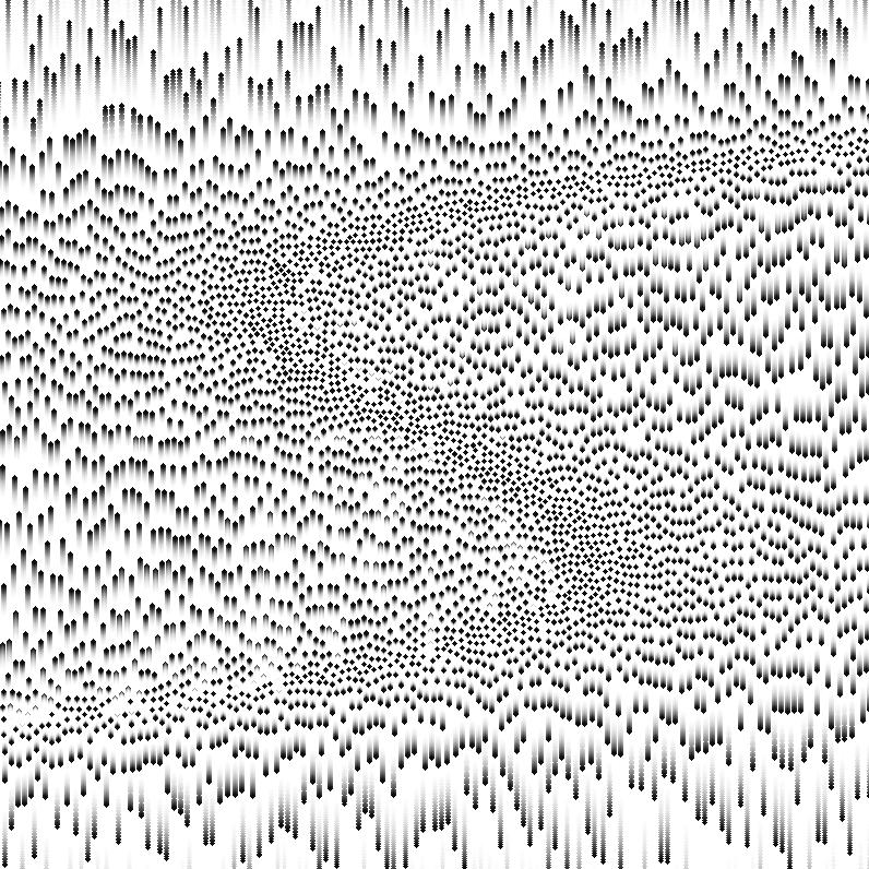
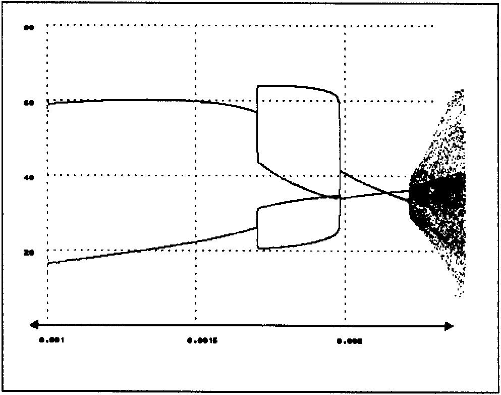
| 1012-Complex.2.jpg, 1013-bif-01.jpg |
| Figure 1.5: (a) Visualizing a local sub-space of interest [44]. (b) Typical bifurcation diagram. | |
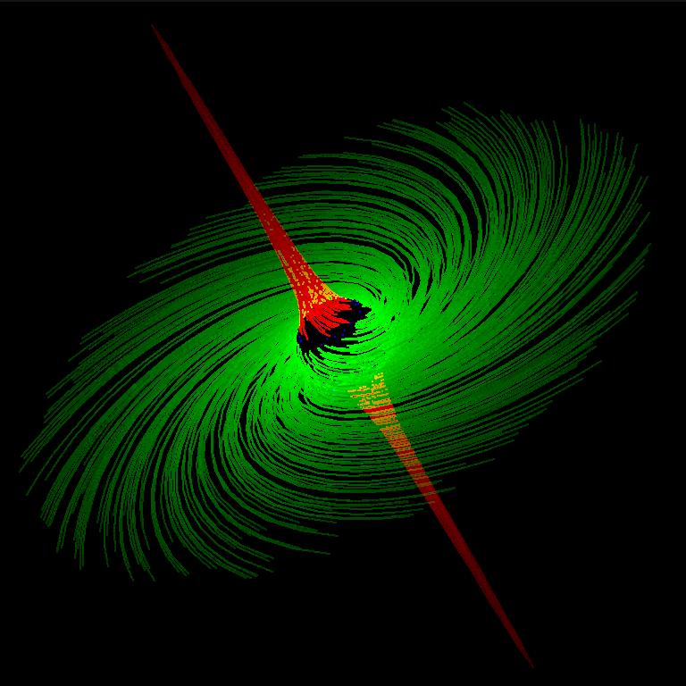
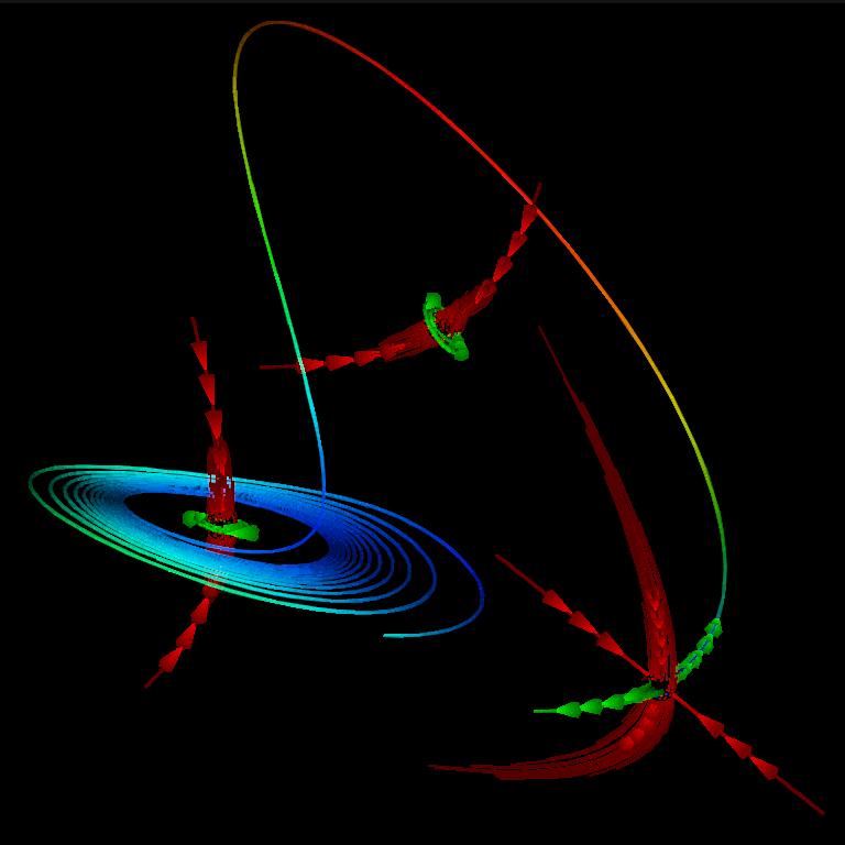
| 1014-Lorenz.2.jpg, 1015-wijk2.jpg |
| Figure 1.6: (a) Visualizing an abstraction of a three-dimensional dynamical system [44]. (b) Visualizing the results of local analysis [19]. | |