|
  | 1016-stro-01.jpg, 1017-stro-02.jpg |
| Figure 2.1: Two examples of visualization used for the communication
of results gained from in-depth analysis of two-dimensional
dynamical systems (images by
Strogatz [80]). |
  | 1018-absh-01.jpg, 1019-absh-02-b.jpg |
| Figure 2.2: Two examples of hand-drawn flow visualization (images
by Abraham and Shaw [1]). |
  | 1020-ex-tex-01.jpg, 1021-ex-tex-03.jpg |
| Figure 2.3: Experimental flow visualization, two
examples [67]:
(a) particles within the flow (image by Delft
Hydraulics) and
(b) shadow graph technique (image
by High-Speed Lab, Dept. of Aerospace Eng., Delft
Univ. of Techn.). |
   |
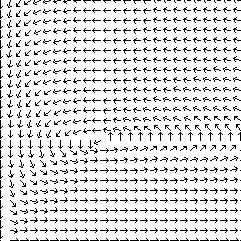
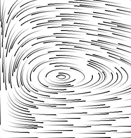
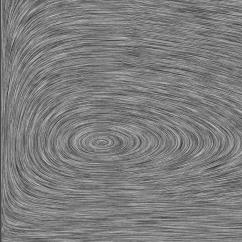
1022-lotvolt-arrows-less.jpg, 1023-lotvolt-frolic-02.jpg, 1024-lotvolt-lic-less.jpg |
| Figure 2.4: Three basic visualization techniques used for the
Lotka-Volterra model:
(a) hedgehog plot,
(b) streamlets, and
(c) LIC. |
  |
1025-isl.jpg,
1026-dipoleV.jpg |
| Figure 2.5: Two examples for rendering stream lines in 3D:
(a) illuminated stream lines
by Zöckler et al. [94], and
(b) vector field rendering by
Banks [8]. |
 | 1027-strribs-01.jpg |
| Figure 2.6: Stream ribbons show the rotation around stream lines
(image by Hans-Georg Pagendarm) [62]. |
  |
1028-strsurf-01.jpg,
1029-flowvol-01.jpg |
| Figure 2.7: (a) Stream surface (image by the Data
Visualization Group, NAS, NASA) [58].
(b) Flow volume (image by the Visualization group
at LLNL) [18]. |
  |
1030-schroe-01.jpg,
1031-schroe-02.jpg |
| Figure 2.8: Two examples for flow visualization by the use of stream
tubes (images by Schröder et al. [75]). |
  |
1032-wijk2.jpg,
1033-freiburg-01.jpg |
| Figure 2.9: (a) Local flow probe by de Leeuw and
van Wijk [19].
(b) Icons for the visualization of local
properties by Happe and Rumpf [74]. |
  |
1034-topo-05.jpg,
1035-topo-01.jpg |
| Figure 2.10: Two examples of the visualization of vector field
topology (images by Helman et
al. [31]). |
 | 1036-tens-03.jpg |
| Figure 2.11: An example for tensor field visualization by Delmarcelle
and Hesselink [21]. |