|
 | 1037-asshaw.jpg |
| (image on first page of Chapt. 4) |
  |
1038-mmo-sl.1.jpg,
1039-figure8.jpg |
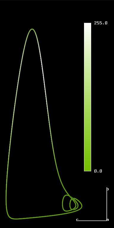
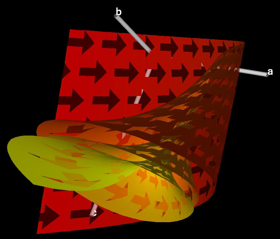
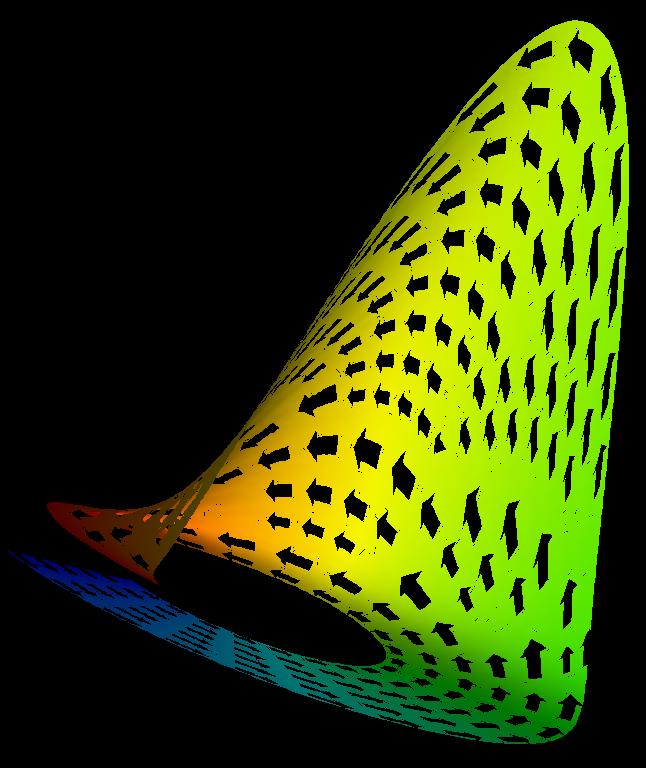
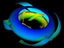
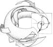
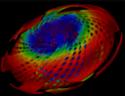
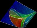
| Figure 4.1: A typical stream line (a)
and stream surface (b)
calculated for a dynamical
system exhibiting mixed-mode oscillations. |
 | 1040-shaw.jpg |
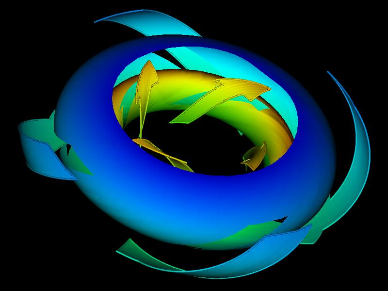
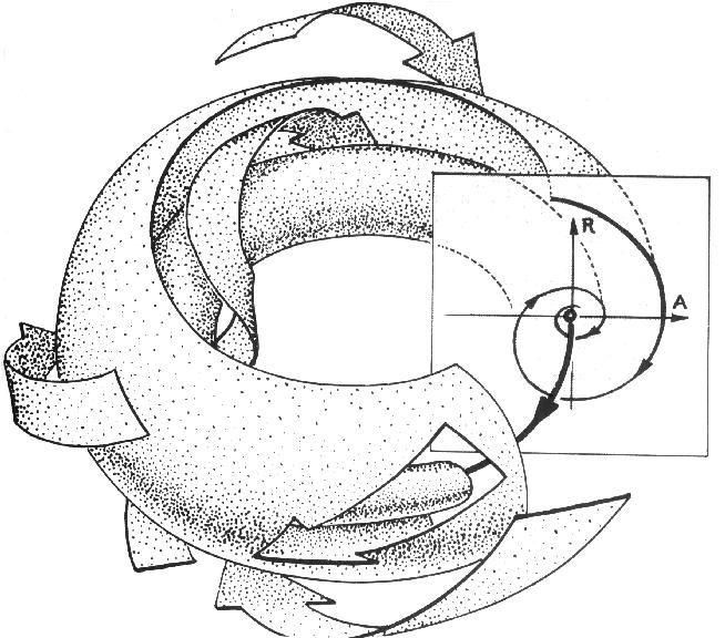
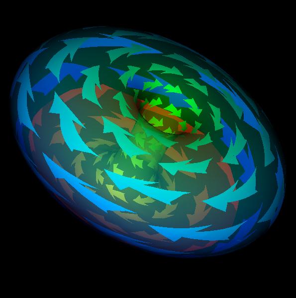
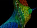
| Figure 4.2: Visualization of a dynamical system by using stream
arrows [1]. |
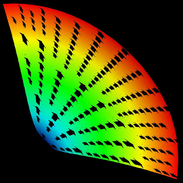
 | 1041-arrows.jpg |
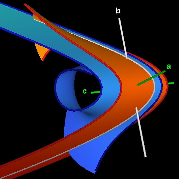
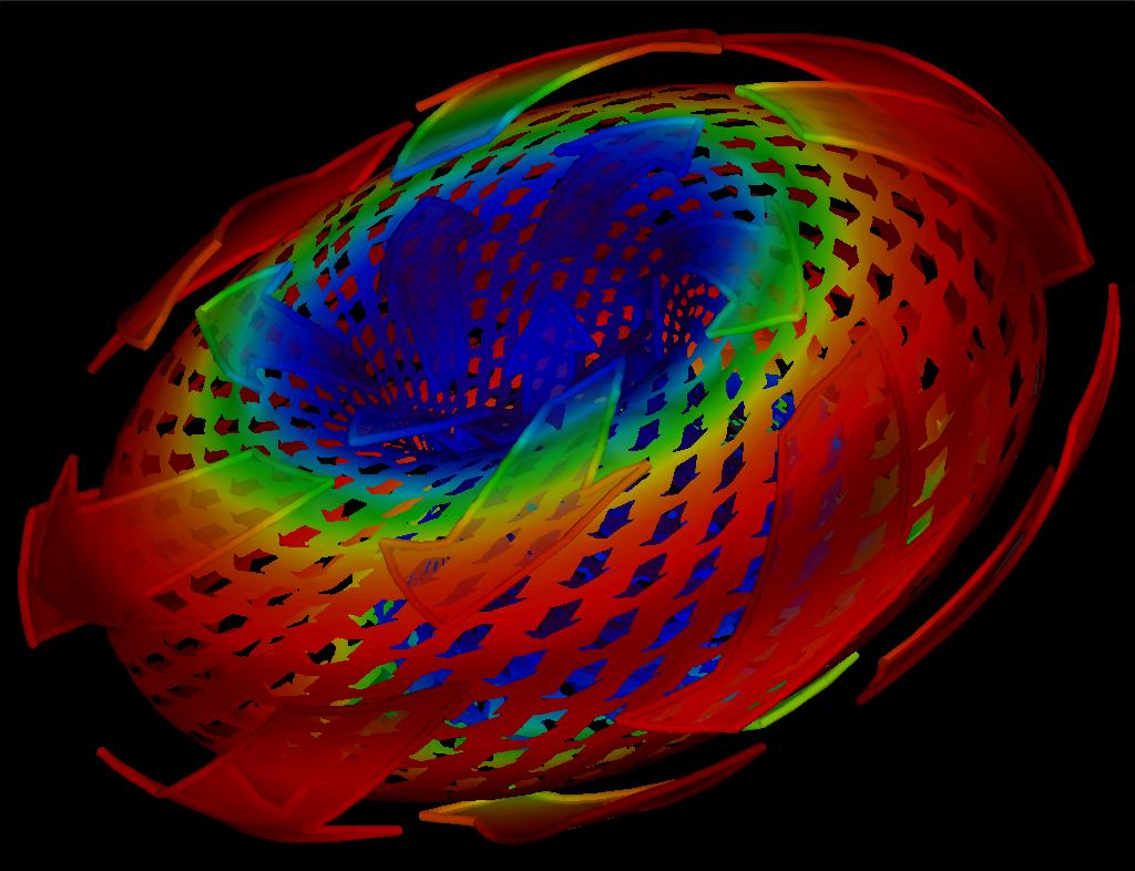
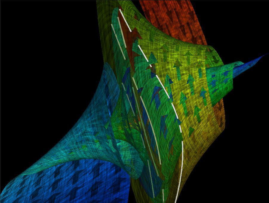
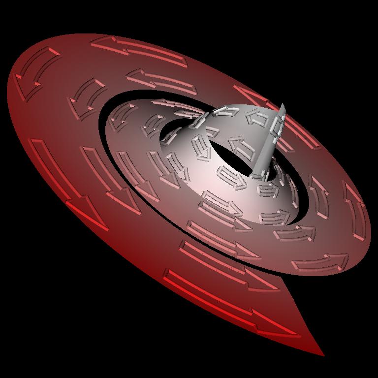
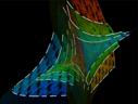
| Figure 4.3: Stream arrows for mixed-mode oscillations. |
  |
1042-shapes1.jpg,
1043-shapes2.jpg |
| Figure 4.4: Varying the shape of the stream arrows texture. [left image] [right image] |
 | 1045-old-arr.gif |
| Figure 4.5: Mapping the stream arrows texture to a stream surface. |
 | 1044-h-arrows.jpg |
| Figure 4.6: Using semi-transparency either for the arrows or the
remaining stream surface portions. |
  |
1046-hierarchical2.jpg,
1047-hierarchical1.jpg |
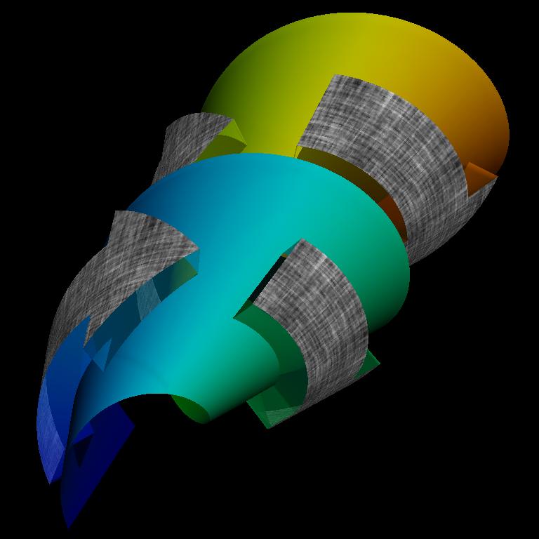
| Figure 4.7: Hierarchical stream arrows, two examples. [left image] [right image] |
 | 1048-h-arr-tex.gif |
| Figure 4.8: Hierarchical stream arrows texture, i.e., a stack of
stream arrows textures - specification
parameters. |
 | 1049-arr-prob.gif |
| Figure 4.9: Activating and locking tiles, example with two triangles. |
  |
1050-spot.jpg,
1051-spot-texture.jpg |
| Figure 4.10: spot (enlarged) and the resulting spot noise
texture. |
 | 1052-texture.jpg |
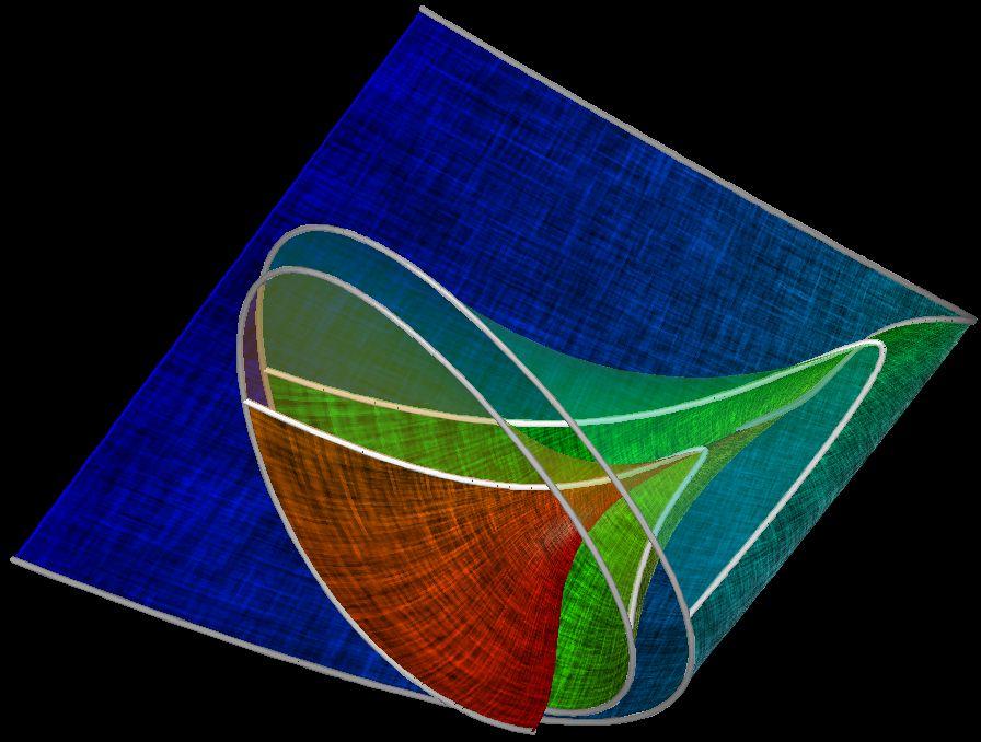
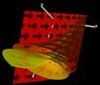
| Figure 4.11: Stream surface with anisotropic spot noise texture. |
  |
1053-result1.jpg,
1054-result2.jpg |
| Figure 4.12: Two snapshots from an animation sequence - the first
from the beginning and the second from the end of the
animation sequence. |
  |
1056-shifted.jpg,
1057-tubearrows.jpg |
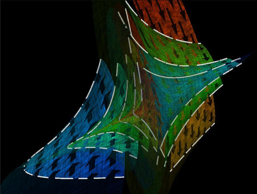
| Figure 4.13: (a) Stream arrows shifted out of the stream surface plus
anisotropic spot-noise.
(b) Stream arrows outlines
represented as 3D tubes and color coding of velocity
magnitude. |
 | 1055-shifted-vs-real2.gif |
| Figure 4.14: Misleading shifted stream arrows (bright: integrated
stream arrow). |