|
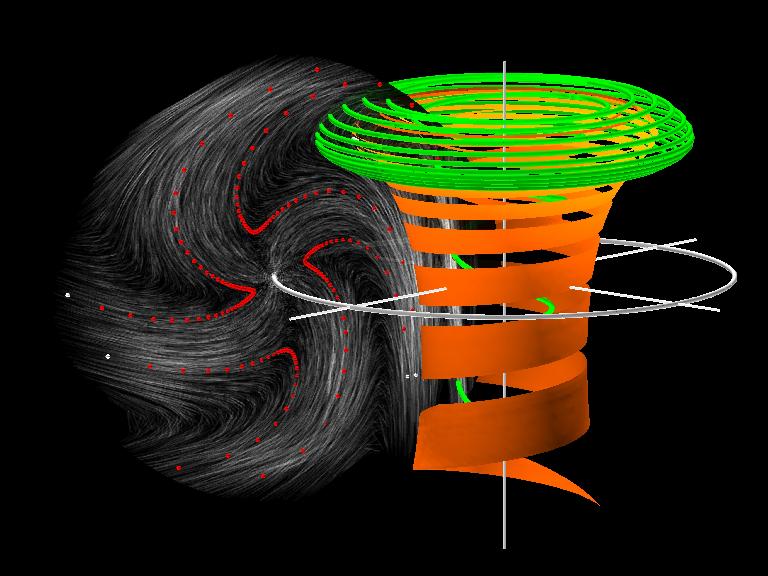
 | 1058-yellowGD36.jpg |
| (image on first page of Chapt. 5) |
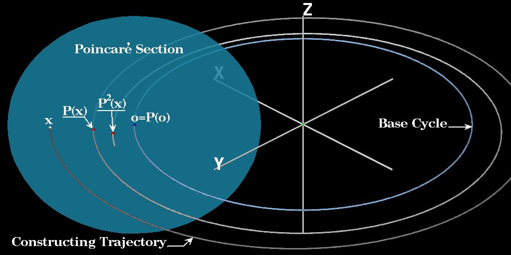
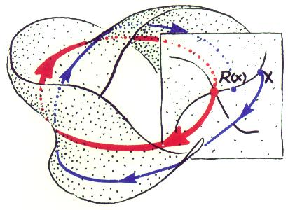
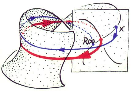
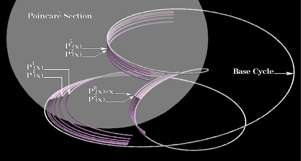
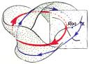
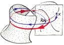
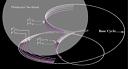
 | 1059-pmexplanation.jpg |
| Figure 5.1: An illustration of the Poincaré map definition. |
  |
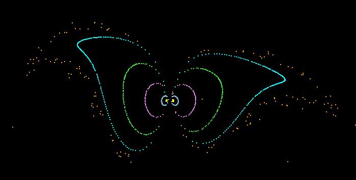
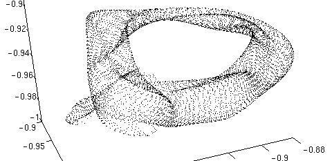
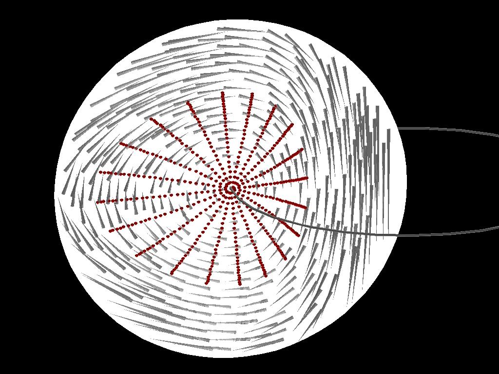
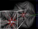
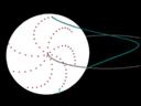
1060-L5Poincare.jpg,
1061-3dpm.jpg |
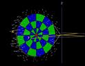
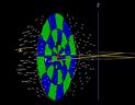
| Figure 5.2: (a) An example of a traditional Poincaré map
visualization [76].
(b) An example of a 3D Poincaré map [15]. |
  |
1062-shaw1.jpg,
1063-shaw2.jpg |
| Figure 5.3: Poincaré map visualization by Abraham and
Shaw [1]. |
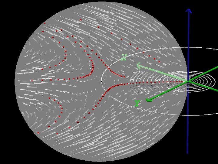
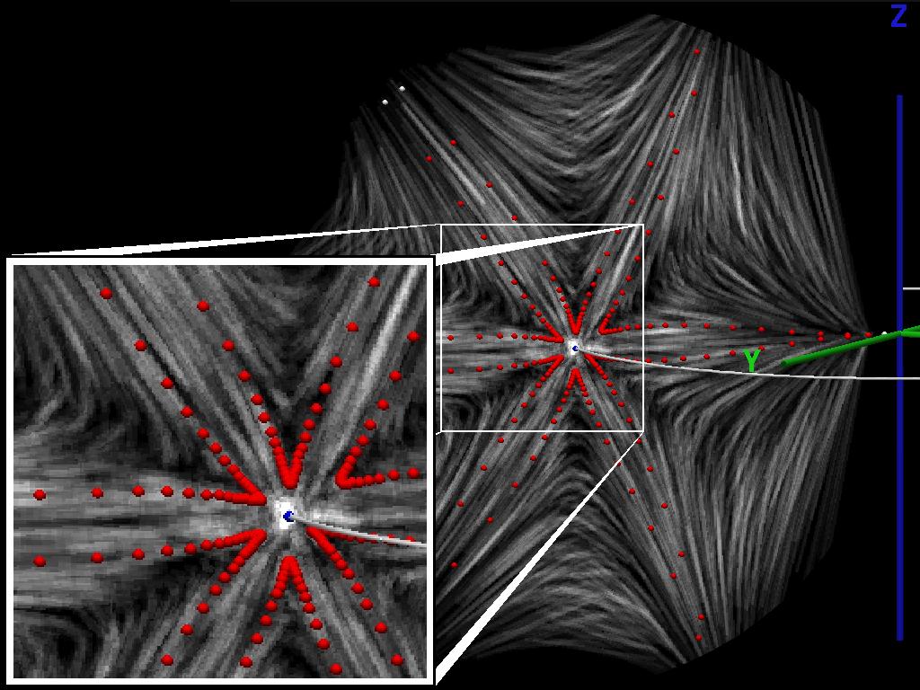
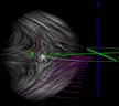
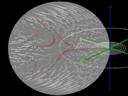 | 1064-ani1.jpg |
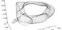
| Figure 5.4: Visualizing a non-linear saddle cycle. |
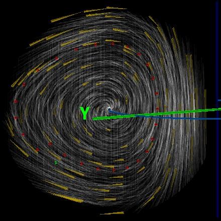
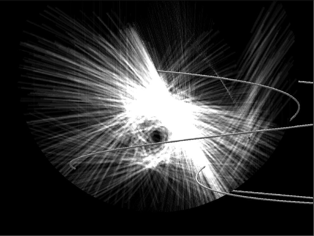
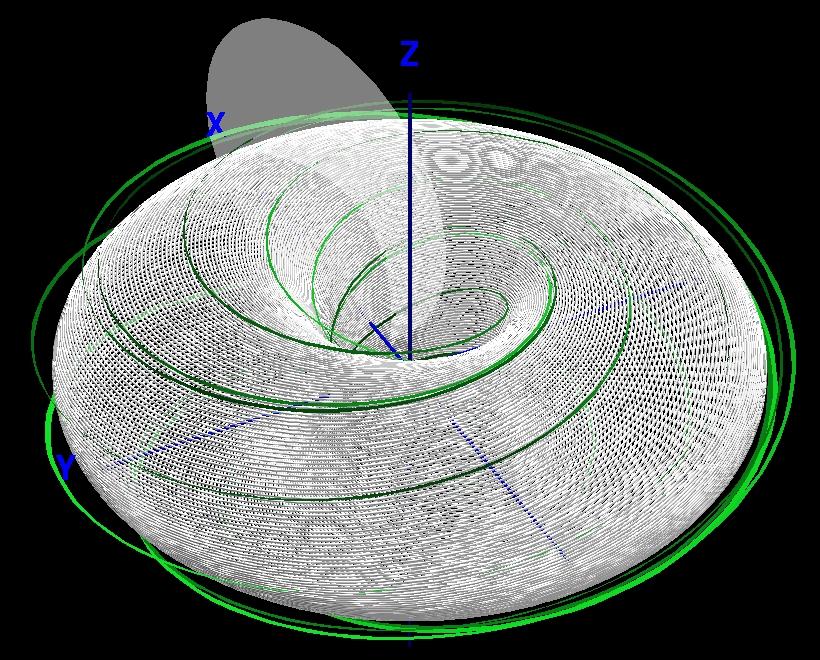
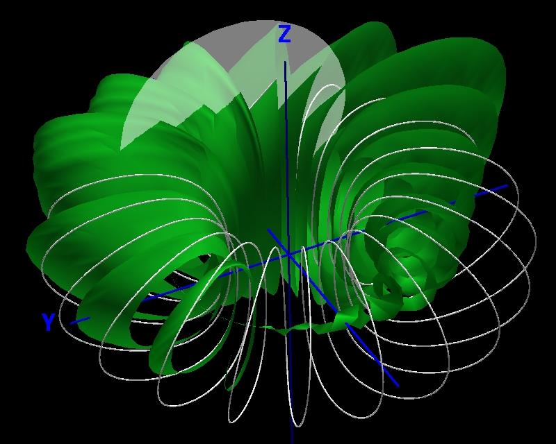
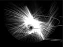
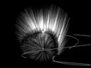
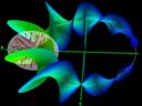
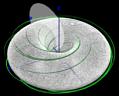
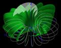
 | 1065-rtorus_flow.jpg |
| Figure 5.5: Visualizing an cycle attractor using spot noise. |
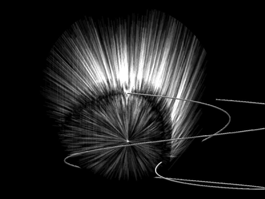
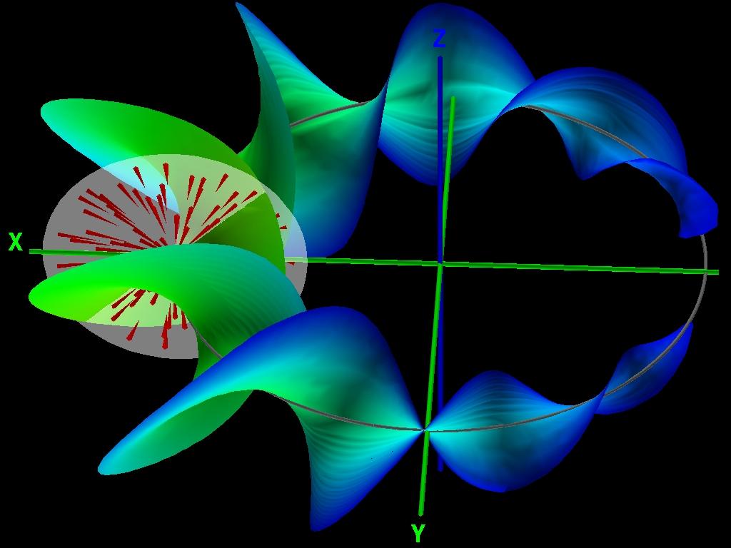
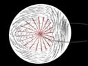
 | 1066-sstpi.jpg |
| Figure 5.6: Visualizing a non-hyperbolic saddle cycle. |
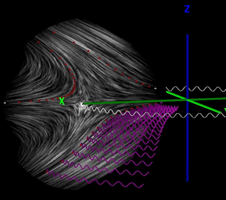
 | 1067-fig-pq.jpg |
| Figure 5.7: Visualizing why
pq is sometimes more
expressive than
p. |
  |
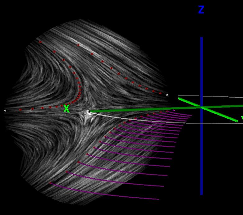
1068-fig-p1.jpg,
1069-fig-p3.jpg |
Figure 5.8: Visualizing
(a)
 vs. (b)
 . . |
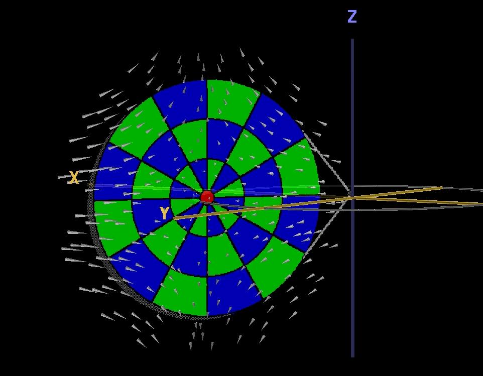
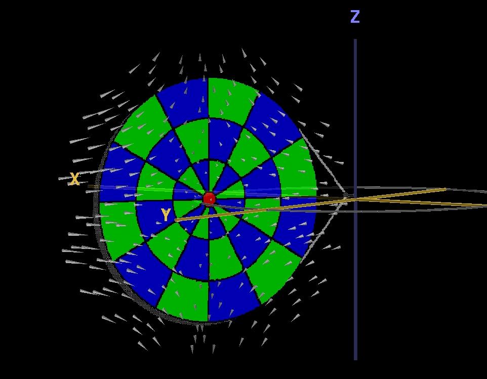
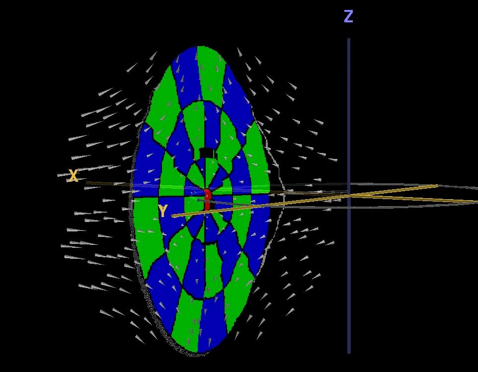
 | 1070-fig-warp.gif |
| Figure 5.9: Evaluating the initial texture after two applications
of
w. |
   |
1074-rc_warp00.jpg,
1075-rc_warp01.jpg,
1076-rc_warp11.jpg |
Figure 5.10: Images resulting from one, two, and eleven applications
of warp function
w, i.e.,
 , ,
 ,
and ,
and
 . . |
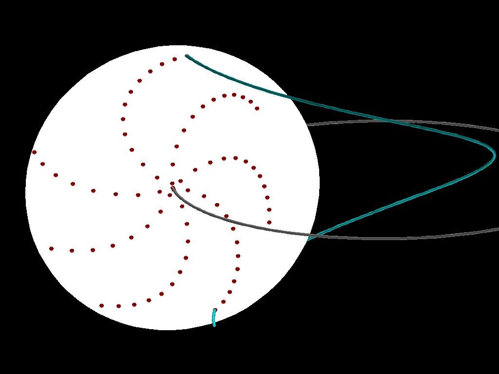
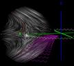
 | 1071-rtorus_seed.jpg |
| Figure 5.11: Visualizing flow properties not encoded within the Poincaré
map. |
  |
1072-zitter1.jpg,
1073-zitter2.jpg |
| Figure 5.12: Visualizing supplementary information in 3D. [left image] [right image] |
  |
1077-rtorus_broken.jpg,
1078-rtorus_green.jpg |
| Figure 5.13: Extreme phase relations as difficult cases for the
visualization of Poincaré maps. [left image] [right image] |
  |
1079-rtorus1_flow_sphere.jpg, 1080-rtorus1_good_PM.jpg |
| Figure 5.14: Combined visualization techniques to disambiguate
results. [left image] [right image] |