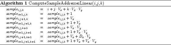
In raycasting the eight samples closest to the current resample location are required in every processing step when trilinear interpolation is used. In a linear volume layout, these samples can be addressed by adding constant offsets to one known address. The necessary address computations are given in Algorithm 1.
![]() are the volume dimensions and
are the volume dimensions and ![]() ,
, ![]() ,
, ![]() are the integer parts of the current resample position. This addressing scheme is very efficient. Once the lower left sample is determined the other needed samples can be accessed just by adding an offset.
are the integer parts of the current resample position. This addressing scheme is very efficient. Once the lower left sample is determined the other needed samples can be accessed just by adding an offset.
The evolution of CPU design shows that the length of CPU pipelines grows progressively. This is very efficient as long as conditional branches do not initiate pipeline flushes. Once a long instruction pipeline is flushed there is a significant delay until it is refilled. Most of the present systems use branch prediction. The CPU normally assumes that if-branches will always be executed. It executes the if-branch before actually checking the outcome of the if-clause. If the if-clause returns false, the else-branch has to be executed. This means that the CPU flushes the pipeline and refills it with the else-branch. This is very time consuming, due to the increasing size of the pipelines.
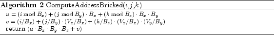
Using a bricked volume layout one will encounter this problem. The addressing of data in a bricked volume layout is more costly than in a linear volume layout. To address one data element, one has to address the block itself and the element within the block. The necessary address computation is given in Algorithm 2. ![]() are block dimensions,
are block dimensions, ![]() are the volume dimensions,
are the volume dimensions, ![]() ,
, ![]() , and
, and ![]() are the integer parts of the current resample position.
are the integer parts of the current resample position.
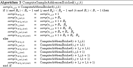
In contrast to this addressing scheme, a linear volume can be seen as one large block. To address a sample it is enough to compute just one offset. In algorithms like volume raycasting, which need to address a certain neighborhood of data in each processing step, the computation of two offsets has a considerable impact on performance. To avoid this performance penalty, one can construct an if-else statement (see Algorithm 3). The if-clause checks if the needed data elements can be addressed within one block. If the outcome is true, the data elements can be addressed as fast as in a linear volume. If the outcome is false, the costly address calculations have to be done. This simplifies address calculation, but the involved if-else statement incurs pipeline flushes. In the following, we address this problem.
|
To avoid the costly if-else statement and the expensive address computations, one can create a lookup table to address all the needed samples. The straight-forward approach would be to create a lookup table for each possible sample position in a block. For a block of ![]() this would lead to
this would lead to ![]() different lookup tables to address the neighboring samples. In the resampling case, 7 neighbors need to be addressed - accordingly the size of the lookup tables would be
different lookup tables to address the neighboring samples. In the resampling case, 7 neighbors need to be addressed - accordingly the size of the lookup tables would be
![]() bytes = 896 KB (4 bytes per offset). For accessing a 26-neighborhood a table of
bytes = 896 KB (4 bytes per offset). For accessing a 26-neighborhood a table of
![]() bytes = 3.25 MB (4 Bytes per offset) would be required. Such a large lookup table is not preferable, due to the limited size of cache. However, the addressing of such a lookup table would be straight-forward, because the indices in the lookup table would be the corresponding offsets of the current sample position, assuming the offset is given relative to the block memory address.
bytes = 3.25 MB (4 Bytes per offset) would be required. Such a large lookup table is not preferable, due to the limited size of cache. However, the addressing of such a lookup table would be straight-forward, because the indices in the lookup table would be the corresponding offsets of the current sample position, assuming the offset is given relative to the block memory address.
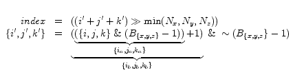
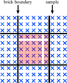
To reduce the size of the lookup table, the possible sample positions can be distinguished by the locations of the needed neighboring samples. The first sample location ![]() is defined by the integer parts of the current resample position. Assuming trilinear interpolation, during resampling neighboring samples to the right, top, and back of the current location are required. A block can be subdivided into subsets. For each subset, we can determine the blocks in which the neighboring samples lie. Therefore, it is possible to store these offsets in a lookup table [9]. This is illustrated in Figure 3.9 (a). We see that there are four basic cases, which can be derived from the current sample location. This can be mapped straightforwardly to 3D, which leads to eight distinct cases. These eight cases are shown in Table 3.2.
is defined by the integer parts of the current resample position. Assuming trilinear interpolation, during resampling neighboring samples to the right, top, and back of the current location are required. A block can be subdivided into subsets. For each subset, we can determine the blocks in which the neighboring samples lie. Therefore, it is possible to store these offsets in a lookup table [9]. This is illustrated in Figure 3.9 (a). We see that there are four basic cases, which can be derived from the current sample location. This can be mapped straightforwardly to 3D, which leads to eight distinct cases. These eight cases are shown in Table 3.2.
In the following, we construct a function to efficiently address the lookup table. The input parameters of the lookup table addressing function are the sample position ![]() and the block dimensions
and the block dimensions ![]() ,
, ![]() , and
, and ![]() . We assume that the block dimensions are a power of two, i.e.,
. We assume that the block dimensions are a power of two, i.e., ![]() ,
, ![]() , and
, and ![]() . As a first step, the block offset parts of
. As a first step, the block offset parts of ![]() ,
, ![]() , and
, and ![]() are extracted by a conjunction with the corresponding
are extracted by a conjunction with the corresponding
![]() . The next step is to increase all by one to move the maximum possible value of
. The next step is to increase all by one to move the maximum possible value of
![]() to
to
![]() . All the other possible values stay within the range
. All the other possible values stay within the range
![]() . Then a conjunction of the resulting value and the complement of
. Then a conjunction of the resulting value and the complement of
![]() is performed, which maps the input values to
is performed, which maps the input values to
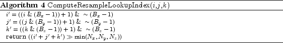
![]() . The last step is to add the three values and divide the result by the minimum of the block dimensions, which maps the result to [0,7]. This last division can be exchanged by a shift operation. Algorithm 4 shows the lookup table index computation and Algorithm 5 shows how the neighboring sample offsets can be computed using the lookup table. We use
. The last step is to add the three values and divide the result by the minimum of the block dimensions, which maps the result to [0,7]. This last division can be exchanged by a shift operation. Algorithm 4 shows the lookup table index computation and Algorithm 5 shows how the neighboring sample offsets can be computed using the lookup table. We use ![]() to denote a bitwise and operation,
to denote a bitwise and operation, ![]() to denote a bitwise or operation,
to denote a bitwise or operation, ![]() to denote a right shift operation, and
to denote a right shift operation, and ![]() to denote a bitwise negation. In Table 3.3 we give an example of the calculation for a block size of
to denote a bitwise negation. In Table 3.3 we give an example of the calculation for a block size of
![]() .
.
|
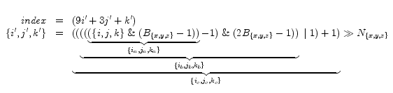
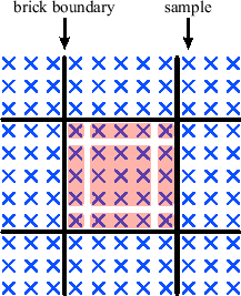
A similar approach can be done for the gradient computation. We present a general solution for a 26-connected neighborhood. Here we can, analogous to the resample case, distinguish 27 cases. For 2D, this is illustrated in Figure 3.9 (b). Depending on the position of sample ![]() a block is subdivided into 27 subsets.
a block is subdivided into 27 subsets.
The first step is to extract the block offset, by a conjunction with
![]() . Then we subtract one, and conjunct with
. Then we subtract one, and conjunct with
![]() , to separate the case if one or more components are zero. In other words, zero is mapped to
, to separate the case if one or more components are zero. In other words, zero is mapped to
![]() . All the other values stay within the range
. All the other values stay within the range
![]() . To separate the case of one or more components being
. To separate the case of one or more components being
![]() , we add 1, after the previous subtraction is undone by a disjunction with 1, without loosing the separation of the zero case. Now all the cases are mapped to
, we add 1, after the previous subtraction is undone by a disjunction with 1, without loosing the separation of the zero case. Now all the cases are mapped to ![]() to obtain a ternary system. This is done by dividing the components by the corresponding block dimensions. These divisions can be replaced by faster shift operations. Then the three ternary variables are mapped to an index in the range of
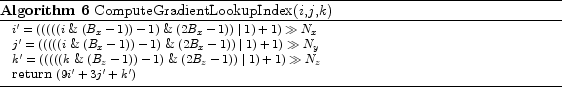
to obtain a ternary system. This is done by dividing the components by the corresponding block dimensions. These divisions can be replaced by faster shift operations. Then the three ternary variables are mapped to an index in the range of ![]() . The final lookup table index computation is given in Algorithm 6. In Table 3.4 we give an example of the calculation for a block size of
. The final lookup table index computation is given in Algorithm 6. In Table 3.4 we give an example of the calculation for a block size of
![]() .
.
The presented index computations can be performed efficiently on current CPUs, since they only consist of simple bit manipulations. The lookup tables can be used in raycasting on a bricked volume layout for efficient access to neighboring samples. The first table can be used if only the eight samples within a cell have to be accessed (e.g., if gradients have been pre-computed). Compared to the if-else solution which has the costly address computation in the else branch, we get a speedup of about 30%. The benefit varies, depending on the block dimensions. For a
![]() block size the else-branch has to be executed in 10% of the cases and for a
block size the else-branch has to be executed in 10% of the cases and for a
![]() block size in 18% of the cases.
block size in 18% of the cases.
The second table allows full access to a 26-neighborhood. This approach reduces the cost of addressing by 40% compared to a if-else solution, as the else-branch has to be executed more often for a larger neighborhood. The lookup table has a size of 27 cases ![]() 26 offsets
26 offsets ![]() 4 bytes per offset = 2808 bytes. This can be reduced by a factor of two due to symmetry reasons. Therefore we have a very small lookup table of 1404 bytes. This is an improvement of a factor of 2427 compared to the straight-forward solution.
4 bytes per offset = 2808 bytes. This can be reduced by a factor of two due to symmetry reasons. Therefore we have a very small lookup table of 1404 bytes. This is an improvement of a factor of 2427 compared to the straight-forward solution.
Another possible option to simplify the addressing is to inflate each block by an additional border of samples from the neighboring blocks [11]. However, such a solution increases the overall memory usage considerably. For example, for a block size of
![]() the total memory is increased by approximately 20%. This is an inefficient usage of memory resources and the storage redundancy reduces the effective memory bandwidth. Our approach practically requires no additional memory, as all blocks share one global address lookup table.
the total memory is increased by approximately 20%. This is an inefficient usage of memory resources and the storage redundancy reduces the effective memory bandwidth. Our approach practically requires no additional memory, as all blocks share one global address lookup table.
![\begin{algorithm}
% latex2html id marker 956\footnotesize
\caption{ComputeSa...
...mple_{i,j,k} + LUT[index][6]$\\
\end{tabular} \end{algorithmic}\end{algorithm}](img162.png)