To demonstrate the impact of our high-level optimizations we used a commodity notebook system equipped with an Intel Centrino 1.6 GHz CPU, 1 MB level 2 cache, and 1 GB RAM. This system has one CPU and does not support Hyper-Threading, so the presented results only reflect performance increases due to our high-level acceleration techniques.
The memory consumption of the gradient cache is not related to the volume dimensions, but determined by the fixed block size. We use
![]() blocks, the size of the gradient cache therefore is is
blocks, the size of the gradient cache therefore is is
![]() byte
byte ![]() 422 KB. Additionally we store for each cache entry a validity bit, which adds up to
422 KB. Additionally we store for each cache entry a validity bit, which adds up to ![]() byte
byte ![]() 4.39 KB.
4.39 KB.
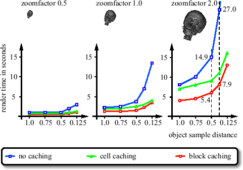
Figure 5.4 shows the effect of per block gradient caching compared to per cell gradient caching and no gradient caching at all. Per cell gradient caching means that gradients are reused for multiple resample locations within a cell. We chose an adequate opacity transfer function to enforce translucent rendering. The charts from left to right show different timings for object sample distances from 1.0 to 0.125 for three different zoom factors 0.5, 1.0, and 2.0. In case of zoom factor 1.0 we have one ray per cell, already here per block gradient caching performs better than per cell gradient caching. This is due to the shared gradients between cells. For zooming out (0.5) both gradient caching schemes perform equally well. The rays are so far apart such that nearly no gradients can be shared. On the other hand, for zooming in (2.0), per block caching performs much better than per cell caching. This is due to the increased number of rays per cell. For this zoom factor, per block gradient caching achieves a speedup of approximately 3.0 compared to no gradient caching at a typical object sample distance of 0.5.
The additional memory usage of the acceleration data structures is rather low. The cell invisibility cache has a size of ![]() bit = 4096 byte. The min-max octree has a depth of three storing 4 byte at each node (a 2 byte minimum and maximum value) and requires at most 2340 byte. Additionally, the classification information is stored, which requires 66 byte. We use blocks of size
bit = 4096 byte. The min-max octree has a depth of three storing 4 byte at each node (a 2 byte minimum and maximum value) and requires at most 2340 byte. Additionally, the classification information is stored, which requires 66 byte. We use blocks of size
![]() storing 2 bytes for each sample, which is a total of 65536 bytes. Our data structures increase the total memory requirements by approximately 10%.
storing 2 bytes for each sample, which is a total of 65536 bytes. Our data structures increase the total memory requirements by approximately 10%.
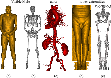
Figure 5.5 compares our acceleration techniques for three large medical datasets. In the fourth column of the table, the render times for entry point determination using block granularity is displayed. Column five shows the render times for octree based entry point determination. In the fifth column, the render times for octree based entry point determination plus cell invisibility caching are displayed. Typically, about 2 frames per second are achieved for these large data sets.
|