The addressing of data in a bricked volume layout is more costly than in a linear volume layout. To address one data element, one has to address the block itself and the element within the block. In contrast to this addressing scheme, a linear volume can be seen as one large block. To address a sample it is enough to compute just one offset. In algorithms like volume raycasting, which need to access a certain neighborhood of data in each processing step, the computation effort for two offsets instead of one generally cannot be neglected. In a linear volume layout, the offsets to neighboring samples are constant. Using bricking, the whole address computation would have to be performed for each neighboring sample that has to be accessed. To avoid this performance penalty, one can construct an if-else statement. The if-clause consists of checking if the needed data elements can be addressed within one block. If the outcome is true, the data elements can be addressed as fast as in a linear volume. If the outcome is false, the costly address calculations have to be done. This simplifies address calculation, but the involved if-else statement incurs pipeline flushes.
We therefore applied a different approach. We distinguished the possible sample positions by the locations of the needed neighboring samples. The first sample location ![]() is defined by the integer parts of the current resample position. Assuming trilinear interpolation, during resampling neighboring samples to the right, top, and back of the current location are required. A block can be subdivided into subsets. For each subset, we can determine the blocks in which the neighboring samples lie. Therefore, it is possible to store these offsets in a lookup table.
is defined by the integer parts of the current resample position. Assuming trilinear interpolation, during resampling neighboring samples to the right, top, and back of the current location are required. A block can be subdivided into subsets. For each subset, we can determine the blocks in which the neighboring samples lie. Therefore, it is possible to store these offsets in a lookup table.
The lookup table contains
![]() offsets. We have eight cases, and for each sample
offsets. We have eight cases, and for each sample ![]() we need the offsets to its seven adjacent samples. The seven neighbors are accessed relative to the sample
we need the offsets to its seven adjacent samples. The seven neighbors are accessed relative to the sample ![]() . Since each offset consists of four bytes the table size is 224 bytes. The basic idea is to extract the eight cases from the current resample position and create an index into a lookup table, which contains the offsets to the neighboring samples.
. Since each offset consists of four bytes the table size is 224 bytes. The basic idea is to extract the eight cases from the current resample position and create an index into a lookup table, which contains the offsets to the neighboring samples.
The input parameters of the lookup table addressing function are the sample position ![]() and the block dimensions
and the block dimensions ![]() ,
, ![]() , and
, and ![]() . We assume that the block dimensions are a power of two, i.e.,
. We assume that the block dimensions are a power of two, i.e., ![]() ,
, ![]() , and
, and ![]() . As a first step, the block offset part from
. As a first step, the block offset part from ![]() ,
, ![]() , and
, and ![]() is extracted by a conjunction with the corresponding
is extracted by a conjunction with the corresponding
![]() . The next step is to increase all by one to move the maximum possible value of
. The next step is to increase all by one to move the maximum possible value of
![]() to
to
![]() . All the other possible values stay within the range
. All the other possible values stay within the range
![]() . Then a conjunction of the resulting value and the complement of
. Then a conjunction of the resulting value and the complement of
![]() is performed, which maps the input values to
is performed, which maps the input values to
![]() . The last step is to add the three values and divide the result by the minimum of the block dimensions, which maps the result to [0,7]. This last division can be exchanged by a shift operation. In summary, the lookup table index for a position
. The last step is to add the three values and divide the result by the minimum of the block dimensions, which maps the result to [0,7]. This last division can be exchanged by a shift operation. In summary, the lookup table index for a position ![]() is given by:
is given by:
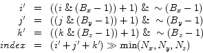 |
(6.1) |
We use ![]() to denote a bitwise and operation,
to denote a bitwise and operation, ![]() to denote a bitwise or operation,
to denote a bitwise or operation, ![]() to denote a right shift operation, and
to denote a right shift operation, and ![]() to denote a bitwise negation.
to denote a bitwise negation.
A similar approach can be done for the gradient computation. We presented a general solution for a 26-connected neighborhood. Here we can, analogous to the resample case, distinguish 27 cases. The first step is to extract the block offset, by a conjunction with
![]() . Then we subtract one, and conjunct with
. Then we subtract one, and conjunct with
![]() , to separate the case if one or more components are zero. In other words, zero is mapped to
, to separate the case if one or more components are zero. In other words, zero is mapped to
![]() . All the other values stay within the range
. All the other values stay within the range
![]() . To separate the case of one or more components being
. To separate the case of one or more components being
![]() , we add 1, after the previous subtraction is undone by a disjunction with 1, without loosing the separation of the zero case. Now all the cases are mapped to
, we add 1, after the previous subtraction is undone by a disjunction with 1, without loosing the separation of the zero case. Now all the cases are mapped to ![]() to obtain a ternary system. This is done by dividing the components by the corresponding block dimensions. These divisions can be replaced by faster shift operations. Then the three ternary variables are mapped to an index in the range of
to obtain a ternary system. This is done by dividing the components by the corresponding block dimensions. These divisions can be replaced by faster shift operations. Then the three ternary variables are mapped to an index in the range of ![]() . In summary, the lookup table index computation for a position
. In summary, the lookup table index computation for a position ![]() is:
is:
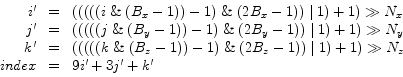 |
(6.2) |
The presented index computations can be performed efficiently on current CPUs, since they only consist of simple bit manipulations. The lookup tables can be used in raycasting on a bricked volume layout for efficient access to neighboring samples. The first table can be used if only the eight samples within a cell have to be accessed (e.g., if gradients have been pre-computed). The second table allows full access to a 26-neighborhood. Compared to the if-else solution which has the costly computation of two offsets in the else branch, we get a speedup of about 30%. The benefit varies, depending on the block dimensions. For a
![]() block size the else-branch has to be executed in 10% of the cases and for a
block size the else-branch has to be executed in 10% of the cases and for a
![]() block size in 18% of the cases.
block size in 18% of the cases.