 |
|
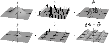
A point sample can be represented as a scaled Dirac impulse function. Sampling a signal is equivalent to multiplying it by a grid of impulses, one at each sample point, as shown in Figure 3.3 [29]. The Fourier transform of a two-dimensional impulse grid with frequency ![]() in
in ![]() and
and ![]() in
in ![]() is itself a grid of impulses with period
is itself a grid of impulses with period ![]() in
in ![]() and
and ![]() in
in ![]() . If we call the impulse grid
. If we call the impulse grid ![]() and the signal
and the signal ![]() , then the Fourier transform of the sampled signal,
, then the Fourier transform of the sampled signal, ![]() , is
, is
![]() . Since
. Since ![]() is an impulse grid, convolving
is an impulse grid, convolving ![]() with
with ![]() amounts to duplicating
amounts to duplicating ![]() at every point of
at every point of ![]() , producing the spectrum shown at bottom right in Figure 3.3. The copy of
, producing the spectrum shown at bottom right in Figure 3.3. The copy of ![]() centered at zero is the primary spectrum, and the other copies are called alias spectra. If
centered at zero is the primary spectrum, and the other copies are called alias spectra. If ![]() is zero outside a small enough region that the alias spectra do not overlap the primary spectrum, then
is zero outside a small enough region that the alias spectra do not overlap the primary spectrum, then ![]() can be recovered by multiplying
can be recovered by multiplying ![]() by a function
by a function ![]() which is one inside that region and zero elsewhere. Such a multiplication is equivalent to convolving the sampled data
which is one inside that region and zero elsewhere. Such a multiplication is equivalent to convolving the sampled data ![]() with
with ![]() , the inverse transform of
, the inverse transform of ![]() . This convolution with
. This convolution with ![]() allows us to reconstruct the original signal
allows us to reconstruct the original signal ![]() by removing, or filtering out, the alias spectra, so we call
by removing, or filtering out, the alias spectra, so we call ![]() a reconstruction filter.
a reconstruction filter.
Thus, the goal of reconstruction is to extract the primary spectrum and to suppress the alias spectra. Since the primary spectrum comprises the low frequencies, the reconstruction filter is a low-pass filter. It is clear from Figure 3.3 that the simplest region to which we could limit ![]() is the region of frequencies that are less than half the sampling frequency along each axis. We call this limiting frequency the Nyquist frequency and the region the Nyquist region. An ideal reconstruction filter can then be defined to have a Fourier transform that has the value one in the Nyquist region and zero outside it.
is the region of frequencies that are less than half the sampling frequency along each axis. We call this limiting frequency the Nyquist frequency and the region the Nyquist region. An ideal reconstruction filter can then be defined to have a Fourier transform that has the value one in the Nyquist region and zero outside it.
Extending the above to three-dimensional signals as used in volume rendering, the sampling grid becomes a three-dimensional lattice and the Nyquist region a cube. Given this Nyquist region, the ideal convolution filter is the inverse transform of a cube, which is the product of three sinc functions.
| (3.1) |
Thus, in principle, a volume signal can be exactly reconstructed from its samples by convolving with ![]() . In practice, however,
. In practice, however, ![]() cannot be implemented, because it has infinite extent in the spacial domain. Practical filters will therefore introduce some artifacts into the reconstructed function. A practical filter takes a weighted sum of a limited number of samples to compute the reconstruction of a point. That is, it is zero outside some finite region. This region is called the region of support. Filters with a larger region of support are generally more expensive since more samples have to be weighted.
cannot be implemented, because it has infinite extent in the spacial domain. Practical filters will therefore introduce some artifacts into the reconstructed function. A practical filter takes a weighted sum of a limited number of samples to compute the reconstruction of a point. That is, it is zero outside some finite region. This region is called the region of support. Filters with a larger region of support are generally more expensive since more samples have to be weighted.
The simplest interpolation function is known as zero-order interpolation, which is actually just a nearest neighbor function. The value at any location is simply the value of the closest sample to that location. One common interpolation function is a piecewise function known as first-order interpolation, or trilinear interpolation. With this function, the value is assumed to vary linearly along directions parallel to one of the major axes. Let the point ![]() lie at location
lie at location
![]() within a cubic cell and let
within a cubic cell and let
![]() be the sample values at the eight corners of the cell. The value
be the sample values at the eight corners of the cell. The value ![]() at location
at location ![]() , according to trilinear interpolation, is then:
, according to trilinear interpolation, is then:
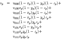 |
(3.2) |
Marschner and Lobb [29] have examined various reconstruction filters. The best results were achieved with windowed sinc filters. While they provide superior reconstruction quality, they are also about two orders of magnitude more expensive than trilinear interpolation. Therefore, when interactive performance is desired, trilinear reconstruction is often the method of choice.