For volume rendering, not only the original function needs to be reconstructed. Especially the first derivative of the three-dimensional function, which is called the gradient, is quite important since it can be interpreted as the normal of an iso-surface. Gradients are used in shading and thus have considerable influence on image quality. Möller et al. [34] even concede gradient reconstruction having a greater impact on image quality than function reconstruction itself. The ideal gradient reconstruction filter is the derivative of the sinc filter, called cosc, which again has infinite extent and therefore cannot be used in practise.
Möller et al. [34] have examined different methods for gradient reconstruction. They have identified the following basic approaches:
In their work, they prove that DF, IF and CD are numerically equivalent and show that the AD method delivers bad results in some cases. An important point of their work is the conclusion that the IF method outperforms the common DF method.
They state that the cost (using caching) of the DF method is
![]() and the cost of the IF method is
and the cost of the IF method is ![]() , where
, where ![]() is the number of voxels,
is the number of voxels, ![]() is the number of samples,
is the number of samples, ![]() is the computational effort of gradient estimation, and
is the computational effort of gradient estimation, and ![]() is the computational effort of the interpolation.
is the computational effort of the interpolation.
However, we recognize that if an expensive gradient estimation method is used, i.e. ![]() is much larger than
is much larger than ![]() , and the sampling rate is high, i.e.
, and the sampling rate is high, i.e. ![]() is much larger than
is much larger than ![]() , the DF method has advantages. Since the gradient estimation only is performed at grid points, a higher sampling rate does not increase the number of necessary gradient estimations. Additionally, from a practical point of view the DF method has other advantages: Modern CPUs provide SIMD extensions which allow to perform operations simultaneously on multiple data items. For the DF method this means that, assuming the same interpolation method is used for gradient and function reconstruction, the interpolation of function value and gradient can be performed simultaneously (i.e., since the function value has to be interpolated anyway, gradient interpolation almost comes for free). Using the IF method, this is not possible, since different filters are used for function and gradient reconstruction.
, the DF method has advantages. Since the gradient estimation only is performed at grid points, a higher sampling rate does not increase the number of necessary gradient estimations. Additionally, from a practical point of view the DF method has other advantages: Modern CPUs provide SIMD extensions which allow to perform operations simultaneously on multiple data items. For the DF method this means that, assuming the same interpolation method is used for gradient and function reconstruction, the interpolation of function value and gradient can be performed simultaneously (i.e., since the function value has to be interpolated anyway, gradient interpolation almost comes for free). Using the IF method, this is not possible, since different filters are used for function and gradient reconstruction.
Central and intermediate differences are two of the most popular gradient estimation methods. However, since they use a small neighborhood they are very sensitive to noise contained in the dataset. Filters which use larger neighborhood therefore in general result in better image quality. This is especially true for medical datasets, which are often strongly undersampled in z-direction.
Neumann et al. [38] have presented a theoretical framework for gradient reconstruction based on linear regression which is a generalization of many previous approaches. The approach linearly approximates the three-dimensional function ![]() according to the following formula:
according to the following formula:
| (3.3) |
The approximation tries to fit a 3D regression hyperplane onto the sampled values assuming that the function changes linearly in the direction of the plane normal ![]() . The value
. The value ![]() is the approximate density value at the origin of the local coordinate system.
They derive a 4D error function and examine its partial derivatives for the four unknown variables. Since these partial derivatives have to equal zero at the minimum location of the error function, they end up with a system of linear equations. Assuming the voxels to be located at regular grid points leads to a diagonal coefficient matrix. Thus, the unknown variables
is the approximate density value at the origin of the local coordinate system.
They derive a 4D error function and examine its partial derivatives for the four unknown variables. Since these partial derivatives have to equal zero at the minimum location of the error function, they end up with a system of linear equations. Assuming the voxels to be located at regular grid points leads to a diagonal coefficient matrix. Thus, the unknown variables ![]() ,
,![]() can be calculated by simple linear convolution:
can be calculated by simple linear convolution:
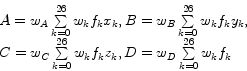 |
(3.4) |
 |
(3.5) |
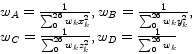
The ![]() are the weights of the weighting function, an arbitrary spherically symmetric function, which is monotonically decreasing as the distance from the local origin is getting larger.
are the weights of the weighting function, an arbitrary spherically symmetric function, which is monotonically decreasing as the distance from the local origin is getting larger. ![]() denotes the index of a voxel with an offset
denotes the index of a voxel with an offset ![]() in the 26-neighborhood of the current voxel and is defined as:
in the 26-neighborhood of the current voxel and is defined as:
| (3.6) |
The vector ![]() is an estimate for the gradient at the local origin and the value
is an estimate for the gradient at the local origin and the value ![]() is the filtered function value at the local origin. Using the filtered values instead of the original samples leads to strong correlation between the data values and the estimated gradients. These low-pass filtered values come as by-product of gradient estimation at little additional cost. Using this estimation method for an arbitrary resample location, however, requires additional computational effort. It is necessary to perform a matrix inversion and a matrix multiplication at each location. Thus, the gradient estimation using Neumann's approach is much cheaper, if gradients are only computed at grid points. However, we do not pre-compute the gradients since this would require a considerable amount of additional memory. Instead, the gradients and filtered values are computed on-the-fly for each cell. Trilinear interpolation is then used to calculate the function value and gradient at each resample location.
is the filtered function value at the local origin. Using the filtered values instead of the original samples leads to strong correlation between the data values and the estimated gradients. These low-pass filtered values come as by-product of gradient estimation at little additional cost. Using this estimation method for an arbitrary resample location, however, requires additional computational effort. It is necessary to perform a matrix inversion and a matrix multiplication at each location. Thus, the gradient estimation using Neumann's approach is much cheaper, if gradients are only computed at grid points. However, we do not pre-compute the gradients since this would require a considerable amount of additional memory. Instead, the gradients and filtered values are computed on-the-fly for each cell. Trilinear interpolation is then used to calculate the function value and gradient at each resample location.
Additionally, this approach has other advantages: Since nothing is pre-computed, different gradient estimation and reconstruction filters can be implemented and simply changed at run-time without requiring further processing. It also helps to solve the problem of using the filtered values instead of the original samples, because the original dataset is still present and the additional filtering can be disabled by the user. This is important in medical applications, since some fine details might disappear due to filtering.