|
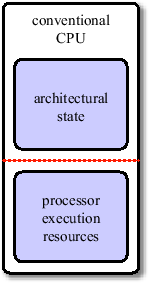
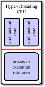
Simultaneous Multithreading is a well-known concept in workstation and mainframe hardware. It is based on the observation that the execution resources of a processor are rarely fully utilized. Due to memory latencies and data dependencies between instructions, execution units have to wait for instructions to finish. While modern processors have out-of-order execution units which reorder instructions to minimize these delays, they rarely find enough independent instructions to exploit the processor's full potential. SMT uses the concept of multiple logical processors which share the resources (including caches) of just one physical processor. Executing two threads simultaneously on one processor has the advantage of more independent instructions being available, and thus leads to more efficient CPU utilization. This can be implemnted by duplicating state registers, which only leads to little increases in manufacturing costs. Intel's SMT implementation is called Hyper-Threading [28] and was first available on the Pentium 4 CPU. Currently, two logical CPUs per physical CPU are supported (see Figure 3.13). Hyper-Threading adds less than 5% to the relative chip size and maximum power requirements, but can provide performance benefits much greater than that.
|
Exploiting SMT, however, is not as straight-forward as it may seem at first glance. Since the logical processors share caches, it is essential that the threads operate on neighboring data items. Therefore, in general, treating the logical CPUs in the same way as physical CPUs leads to little or no performance increase. Instead, it might even lead to a decrease in performance, due to cache thrashing. Thus, our processing scheme has to be extended in order to allow multiple threads to operate within the same block.
The blocks are distributed among physical processors as described in the previous section. Additionally, within a block, multiple threads each executing on a logical CPU simultaneously process the rays of a block. Using several threads to process the ray list of a block would lead to race conditions and would therefore require expensive synchronization. Thus, instead of each block having just one ray list for every physical CPU, we now have
![]() lists per physical CPU, where
lists per physical CPU, where
![]() is the number of threads that will simultaneously process the block, i.e., the number of logical CPUs per physical CPU. Thus, each block has
is the number of threads that will simultaneously process the block, i.e., the number of logical CPUs per physical CPU. Thus, each block has
![]() ray lists
ray lists
![]() where
where ![]() identifies the physical CPU and
identifies the physical CPU and ![]() identifies the logical CPU relative to the physical CPU. A ray can move between physical CPUs depending on how the block lists are partitioned within in each pass, but they always remain in a ray list with the same
identifies the logical CPU relative to the physical CPU. A ray can move between physical CPUs depending on how the block lists are partitioned within in each pass, but they always remain in a ray list with the same ![]() . This means that for equal workloads between threads, the rays have to be initially distributed among these lists, e.g., by alternating the
. This means that for equal workloads between threads, the rays have to be initially distributed among these lists, e.g., by alternating the ![]() of the list a ray is inserted into during ray setup.
of the list a ray is inserted into during ray setup.
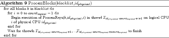
The basic algorithm described in the previous section is extended in the following way: The ProcessBlocks procedure (see Algorithm 9) now starts the execution of ![]() for each logical CPU of the physical CPU it is executed on. ProcessRays (see Algorithm 10) processes the rays of a block for one logical CPU. All other routines remain unchanged.
for each logical CPU of the physical CPU it is executed on. ProcessRays (see Algorithm 10) processes the rays of a block for one logical CPU. All other routines remain unchanged.
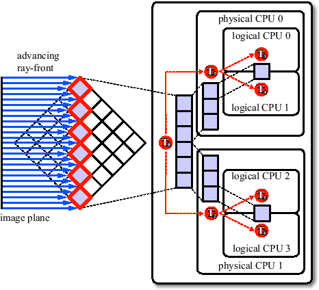
Figure 3.14 depicts the operation of the algorithm for a system with two physical CPUs, each allowing simultaneous execution of two threads, i.e.
![]() and
and
![]() . In the beginning seven treads,
. In the beginning seven treads, ![]() , are started.
, are started. ![]() performs all the preprocessing. In particular, it has to assign the rays to those blocks through which the rays enter the volume first. Then it has to choose the lists of blocks which can be processed simultaneously, with respect to the eight to distinguish viewing directions. Each list is partitioned by
performs all the preprocessing. In particular, it has to assign the rays to those blocks through which the rays enter the volume first. Then it has to choose the lists of blocks which can be processed simultaneously, with respect to the eight to distinguish viewing directions. Each list is partitioned by ![]() and sent to
and sent to ![]() and
and ![]() . After a list is sent,
. After a list is sent, ![]() sleeps until its slaves are finished. Then it continues with the next pass.
sleeps until its slaves are finished. Then it continues with the next pass. ![]() sends one block after the other to
sends one block after the other to ![]() and
and ![]() .
. ![]() sends one block after the other to
sends one block after the other to ![]() and
and ![]() . After a block is sent, they sleep until their slaves are finished. Then they send the next block to process, and so on.
. After a block is sent, they sleep until their slaves are finished. Then they send the next block to process, and so on. ![]() ,
, ![]() ,
, ![]() , and
, and ![]() perform the actual raycasting. Thereby
perform the actual raycasting. Thereby ![]() and
and ![]() simultaneously process one block, and
simultaneously process one block, and ![]() and
and ![]() simultaneously process one block.
simultaneously process one block.
 |
![\begin{algorithm}
% latex2html id marker 1128\footnotesize
\caption{ProcessR...
...[id_{logical}]$,$r$)
\ENDIF
\ENDFOR
\ENDFOR
\end{algorithmic}\end{algorithm}](img203.png)