Gradient Cache

It has been argued that the quality of the final image is heavily influenced by the gradients used in shading [34]. High-quality gradient estimation methods have been developed, which generally consider a large neighborhood of samples. This implies higher computational costs. Due to this, many approaches use expensive gradient estimation techniques to pre-compute gradients at the grid points and store them together with the original samples. The additional memory requirements, however, limit the practical application of this approach. For example, using 2 bytes for each component of the gradient increases the size of the dataset by a factor of four (assuming 2 bytes are used for the original samples). In addition to the increased memory requirements of pre-computed gradients, this approach also reduces the effective memory bandwidth. We therefore choose to perform gradient estimation on-the-fly. Consequently, when using an expensive gradient estimation method caching of intermediate results is inevitable if high performance has to be achieved. An obvious optimization is to perform gradient estimation only once for each cell. When a ray enters a new cell, the gradients are computed at all eight corners of the cell. These gradients are then re-used during resampling within the cell. The benefit of this method is dependent on the number of resample locations per cell, i.e., the object sample distance.

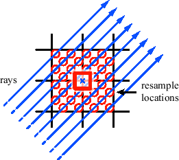
However, the computed gradients are not reused for other cells. This means that each gradient typically has to be computed eight times, as illustrated in Figure 3.15. For expensive gradient estimation methods, this can considerably reduce the overall performance. It is therefore important to store the results in a gradient cache. However, allocating such a cache for the whole volume still has the mentioned memory problem.

Our blockwise volume traversal scheme allows us to use a different approach. We perform gradient caching on a block basis. Our cache is capable of storing one gradient for every grid point of a block. Thus, the required cache size is $(B_x + 1) \times (B_y + 1) \times (B_z + 1)$ where $B_x$, $B_y$, $B_z$ are the block dimensions. The block dimensions are increased by one to enable interpolation across block boundaries. Each entry of the cache stores the three components of a gradient, using a single precision floating-point number for each component. Additionally, a bit set has to be stored that encodes the validity of an entry in the cache for each grid point of a block.

When a ray enters a new cell, for each of the eight corners of the cell the bit set is queried. If the result of a query is zero, the gradient is computed and written into the cache. The corresponding value of the bit set is set to one. If the result of the query is one, the gradient is already present in the cache and is retrieved.

The disadvantage of this approach is that gradients at block borders have to be computed multiple times. However, this caching scheme still greatly reduces the performance impact of gradient computation and requires only a modest amount of memory. Furthermore, the required memory is independent of the volume size, which makes this approach applicable to large datasets.

Figure 3.15: Redundant gradient computation at grid positions. Without caching, the gradient at the highlighted grid position has to be recomputed multiple times.