Entry Point Buffer

One of the major performance gains in volume rendering can be achieved by quickly skipping data which is classified as transparent. In particular, it is important to begin sampling at positions close to the data of interest, i.e., the non-transparent data. This is particularly true for medical datasets, as the data of interest is usually surrounded by large amounts of empty space (air). The idea is to find, for every ray, a position close to its intersection point with the visible volume, thus, we refer to this search as entry point determination. The advantage of entry point determination is that it does not require additional overhead during the actual raycasting process, but still allows to skip a high percentage of empty space. The entry points are determined in the ray setup phase and the rays are initialized to start processing at the calculated entry position. The basic goal of entry point determination is to establish a buffer, the entry point buffer, which stores the position of the first intersection with the visible volume for each ray.

As blocks are the basic processing units of our algorithm, the first step is to find all blocks which do not contribute to the visible volume using the current classification, i.e., all blocks that only contain data values which are classified as transparent. It is important that the classification of a whole block can be efficiently calculated to allow interactive transfer function modification. We store the minimum and maximum value of the samples contained in a block and use a summed area table of the opacity transfer function to determine the visibility of the block [19].

A summed area table is a data structure for integrating a discrete function. We use a one-dimensional summed area table to evaluate the integral of the opacity transfer function $\alpha$ over the voxels represented by a block. The summed area table is computed in the following way: $S(0)$ is equal to $\alpha (0)$ and $S(i)$ = $S(i-1) + \alpha (i)$ for all $i > 0$.

The integral of the discrete function $\alpha$ over the interval $[i_{min},i_{max}]$ can then be evaluated in constant time by performing two table lookups:

$$\sum\limits_{i_{\min } }^{i_{\max } } {\alpha (i) = S(i_{\max } ) - S(i_{\min } - 1)}$$ (3.14)

Figure 3.16: Block template generation. The block is projected onto the image plane, its depth values are rasterized and stored in a template image.

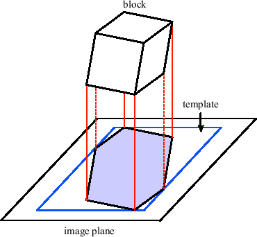We then perform a projection of each non-transparent block onto the image plane with hidden surface removal to find the first intersection point of each ray with the visible volume [49]. The goal is to establish an entry point buffer of the same size as the image plane, which contains the depth value for each ray's intersection point with the visible volume. For parallel projection, this step can be simplified. As all blocks have exactly the same shape, it is sufficient to generate one template by rasterizing one block under the current viewing transformation (see Figure 3.16). Projection is then performed by translating the template by a vector $t = (t_x,t_y,t_z)^T$ which corresponds to the block's position in three-dimensional space in viewing coordinates. Thus, $t_x$ and $t_y$ specify the position of the block on the image plane (and therefore the location where the template has to be written into the entry point buffer) and $t_z$ is added to the depth values of the template. The Z-buffer algorithm is used to ensure correct visibility. During ray setup, the depth values stored in the entry point buffer are used to initialize the ray positions.

The disadvantage of this approach is that it requires an addition and a depth test at every pixel of the template for each block. This can be greatly reduced by choosing an alternative method. The blocks are projected in back-to-front order. The back-to-front order can be easily established by traversing the generated block lists (see Section 3.3.3) in reverse order. For each block the Z-value of the generic template is written into the entry point buffer together with a unique index of the block. After the projection has been performed, the entry point buffer contains the indices and relative depth values of the entry points for each ray. During ray setup, the block index is used to determine the translation vector $t$ for the block and $t_z$ is added to the relative depth value stored in the buffer to find the entry point of the ray. The addition only has to be performed for every ray that actually intersects the visible volume.

Figure 3.17: Block and octree projection. (a) projection of non-transparent blocks. (b) projection of non-transparent octree nodes.

(a)	(b)

We further extend this approach to determine the entry points in a higher resolution than block granularity. We replace the minimum and maximum values stored for every block by a min-max octree. Its root node stores the minimum and maximum values of all samples contained in a block. Each additional level contains the minimum and maximum value for smaller regions, resulting in a more detailed description of parameter variations inside the block. The resulting improvement in entry point determination is depicted in Figure 3.17.

The advantage of a min-max octree is, that it stores only information about the data values, which are independent of the transfer functions and viewing parameters. Thus, the octree can be generated in a preprocessing step. When the classification changes, the summed area table is used to efficiently determine the visibility of each octree node.

For determining the visibility of an octree node, the integral over the interval defined by the minimum and maximum values of the node is evaluated using the summed area table. If the integral is zero, then all voxels represented by the node are transparent. Otherwise, a more detailed level of the octree is used to refine the estimated classification.

When the classification changes, the summed-area table is recursively evaluated for all blocks. The classification information itself can be stored efficiently using a technique called hierarchy compression. Our octree has a maximum depth of three for each block. All nodes except the most detailed octree level (level 2) have three states (see Figure 3.18):

• opaque, i.e., none of the children of the node is transparent,
• transparent, i.e., all of the node's children are transparent,
• inhomogeneous, i.e., the node has transparent and non-transparent children.

Figure 3.18: Octree classification of a block. The block is recursively subdivided into nodes which are either classified as fully transparent, fully opaque, or inhomogeneous. Leaf nodes can only be fully transparent or fully opaque.

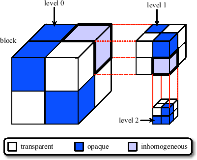For efficient storage and visibility determination, we use the following scheme: The information whether a node of level 2 is transparent or opaque is stored in one bit. Since each node of level 1 contains eight nodes of level 2, no additional information has to be stored for level 1. The state of a level 1 node can be determined by testing the byte which contains all the bits of its children. For level 0 such a hierarchy compression scheme would require to test 8 bytes to determine the state of a level 0 node and 64 bytes for the whole block. Thus, for level 0 we explicitly store the state information. Since there are three states, we need two bits for each level 0 node. Thus, two additional bytes are stored which contain the two bit state information for all level 0 nodes.

The projection algorithm is modified as follows. Instead of one block template there is now a template for each octree level. The projection of one block is performed by recursively traversing the hierarchical classification information in back-to-front order and projecting the appropriate templates for each level, if the corresponding octree node is non-transparent. In addition to the block index, the entry point buffer also stores an index for the corresponding octree node (node index). During ray setup, the depth value in the entry point buffer is translated by the $t_z$ component of the translation vector plus the sum of the relative offsets of the node in the octree.

The node index encodes the position of a node's origin within the octree. It can be calculated in the following way:

$$index(node) = \sum\limits_{i = 0}^{N-1} {octant_i(node) \cdot 8^{N - i - 1} }$$ (3.15)

where $N$ is the depth of the octree, $octant_i$ is the octant of level $i$ where the node is located. For an octree of depth $N$ there are $8^{N}$ different indices. The relative translational offsets for the octree nodes can be pre-computed and stored in a lookup table of $8^{N}$ entries indexed by the node index.