We also adapted spot noise [87] to Poincaré maps. We
place elliptic spots onto
![]() such that the focal points
of the ellipses coincide with
xi and
p(xi), respectively. See Fig. 5.5 for an
example.
This choice is due to the fact that no directional information
should be encoded, when
p(xi)=
xi. In
this case both focal points coincide and the elliptic spot
degenerates to a circular spot. Images rendered with this method are
well suited to visualize the entirety of
such that the focal points
of the ellipses coincide with
xi and
p(xi), respectively. See Fig. 5.5 for an
example.
This choice is due to the fact that no directional information
should be encoded, when
p(xi)=
xi. In
this case both focal points coincide and the elliptic spot
degenerates to a circular spot. Images rendered with this method are
well suited to visualize the entirety of
![]() within
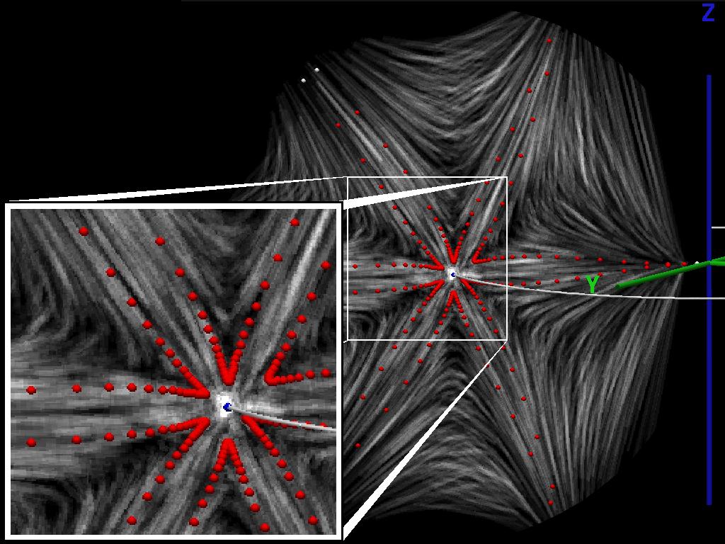
one still image. See Fig. 5.6 for a visualization of a
non-hyperbolic saddle cycle (3 stable and 3 unstable manifolds)
where spot noise was used for visualization. Similar as in
Fig. 5.4, six
sequences
within
one still image. See Fig. 5.6 for a visualization of a
non-hyperbolic saddle cycle (3 stable and 3 unstable manifolds)
where spot noise was used for visualization. Similar as in
Fig. 5.4, six
sequences
![]() are visualized by the use of white and red spheres.
are visualized by the use of white and red spheres.
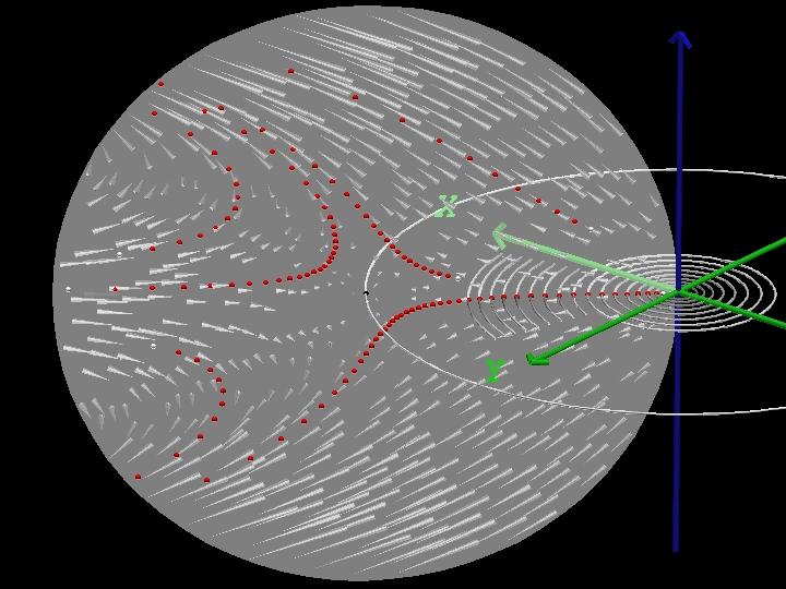
The results of the previous techniques are now embedded into a
3D visualization of the underlying flow. We therefore represent
Poincaré section
![]() as a semi-transparent disk placed
within the flow and realize the arrows and spot noise as a
texture of this disk (see Figs. 5.4 and 5.6).
Semi-transparency was used for the map to allow the viewer to see
through. This improves the understanding of the context of
map
p.
as a semi-transparent disk placed
within the flow and realize the arrows and spot noise as a
texture of this disk (see Figs. 5.4 and 5.6).
Semi-transparency was used for the map to allow the viewer to see
through. This improves the understanding of the context of
map
p.
![\framebox[\textwidth]{
\includegraphics[width=.93\textwidth]{pics/ani1.ps}
}](img191.gif)
![\framebox[\textwidth]{
\includegraphics[width=.93\textwidth]{pics/rtorus_flow.ps}
}](img194.gif)
![\framebox[\textwidth]{
\includegraphics[width=.93\textwidth]{pics/sstpi.ps}
}](img197.gif)