Visualizing the repeated application  pⁿ

There are several reasons to investigate the repeated application of Poincaré map  p, i.e.,  pⁿ. Probably the most important one is the analysis of the asymptotic behavior induced by the (iterated) Poincaré map. Periodic systems near a cycle can exhibit different asymptotic behavior, e.g., convergence or divergence with respect to the cycle. This aspect is due to different possible cycle characteristics, namely stable, saddle, or unstable behavior. A stable cycle attracts near trajectories, whereas unstable and saddle cycles repel near trajectories. A saddle cycle  $\mathcal{C}$ separates its Poincaré section  $\mathcal{S}$ into regions of attraction and regions of repulsion. Almost all trajectories near  c= p(c) emerge into the repelling parts of $\mathcal{S}$ and thus are finally repelled from  $\mathcal{C}$. Figs. 5.4 and 5.6 show two Poincaré maps of different saddle cycles.

We implemented a module TRAJECTORY which produces a visualization of the set  $\left\{\mathbf{p}^j(\mathbf{x})\ \vert\ j\!\ge\!0\right\}$ as described on page . See Fig. 5.6 for another example where this technique was used.

  

Figure 5.7: Visualizing why p^q is sometimes more expressive than  p.

  

Figure 5.8: Visualizing  (a)  $\{(\mathbf{x}_i,\mathbf{p}(\mathbf{x}_i))\}$ vs.  (b)  $\{(\mathbf{x}_i,\mathbf{p}^3(\mathbf{x}_i))\}$.

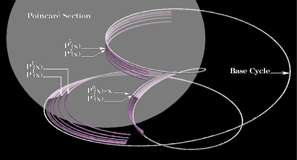
Sometimes p^q, q>1, is more interesting to investigate than  p. This is the case, for example, when base cycle  $\mathcal{C}$ itself pierces the Poincaré section q times during one complete loop (see Fig. 5.7). In the given example $\mathcal{C}$ intersects $\mathcal{S}$ two more times before it returns to the initial intersection point and thus closes the cycle. The behavior of trajectories  $\mathcal{T}$ near $\mathcal{C}$ are better described by one arbitrary  $\mathbf{x}\!\in\!\mathcal{T}\!\cap\!\mathcal{S}$ and p³(x) rather than  x and p(x). In fact any pair  $(\mathbf{p}^j(\mathbf{x}),\,\mathbf{p}^{j+q}(\mathbf{x}))$, 0$\le$j<q, can be chosen for this type of analysis.

The user can change the default value of q, i.e., 1, such that all the previously discussed visualization techniques, e.g., spot noise, are adapted to this new parameter setting. Moreover we allow the user to specify that only those intersections  $\mathbf{y}\!=\!\mathcal{T}$$\cap$ $\mathcal{S}$ are considered where $\mathbf{f}(\mathbf{y})\!\cdot\!\mathbf{f}(\mathcal{C}\!\cap\!\mathcal{S})>0$ ( f being the underlying 3D flow). Only those points on trajectory $\mathcal{T}$ are of interest where $\mathcal{T}$ crosses the Poincaré section with the same orientation. This means that $\mathcal{T}$ crosses $\mathcal{S}$ in both cases either in front-to-back or back-to-front orientation. Fig. 5.8(a) was rendered with q=1 and Fig. 5.8(b) with q=3. In this case the base cycle pierces $\mathcal{S}$ three times during one complete loop.

Although there are still some artifacts in Fig. 5.8(b) which are due to the limited size of $\mathcal{S}$, it is more expressive than Fig. 5.8(a). The egg-shaped intersection of an invariant torus (containing the base cycle) and Poincaré section  $\mathcal{S}$ can be clearly seen as dark line around the center of this image. Furthermore the unstable cycle within this torus cross-section can be distinguished as a critical point of the Poincaré map  p. The radial repulsion away from this critical point towards the torus is well represented by the star like spot noise texture.

The visualization of pⁿ, n>1, is more difficult than visualizing p itself. A technique we investigated for the representation of pⁿ, n increasing, is image warping [11]. A module WARP was implemented that approximates p by a warp function  w on the basis of $\mathcal{L}$ and $\mathbf{p}(\mathcal{L})$ where $\mathcal{L}$ can be chosen to be either a jittered or regular set of line segments spread over  $\mathcal{S}$. This approximation is necessary since evaluating the Poincaré map for all the points on the Poincaré section would cause extremely high computational efford - for each single evaluation potentially thousands up to millions of numerical integration steps are necessary - thus only a few evaluations are done, i.e., $\mathbf{p}(\mathcal{L})$, and warping is used to approximate pⁿ.

WARP loads an initial texture $\mathit{TEX}$ onto $\mathcal{S}$ and then applies the warp transformation n times, where n is specified via a parameter of WARP. The resulting texture  $\mathit{TEX}$$\circ\,$ w^-n (see Fig. 5.9) placed on $\mathcal{S}$ gives a good impression of the main characteristics of  pⁿ. See Fig. 5.10 for an images rendered using this technique.

  

Figure 5.9: Evaluating the initial texture after two applications of  w.

  

Figure 5.10: Images resulting from one, two, and eleven applications of warp function  w, i.e., $\mathbf{w}(\mathcal{S})$, $\mathbf{w}^2(\mathcal{S})$, and  $\mathbf{w}^{11}(\mathcal{S})$.

The reason why we approximate Poincaré map  p by the use of a warping function instead of using p directly for the transformation of the texture is that p is usually rather costly to compute. Warp function WARP, on the other hand, is capable of approximating p quite good if warping parameters are chosen appropriately. At least an idea of pⁿ is gained using this technique.

mailto:helwig@cg.tuwien.ac.at.